---
title: "Italian Temperatures, 2006–2023: A Climate Data Story"
description: "From a wide ISTAT workbook to tidy data, trend estimates, and matplotlib charts styled to match the blog for Italian provincial capitals."
author: "Federico Viscioletti"
date: "2026-07-02"
lang: en
categories: [data-science, python, climate, data-visualization]
pillar: data-science-insights
cluster: data-cleaning
pillar-stage: case-study
image: "images/italian-temperatures-analysis.png"
jupyter: python3
translations:
es: /posts/2026/07/02/analisis-de-temperaturas-italianas-2006-2023/
fr: /posts/2026/07/02/temperatures-italiennes-2006-2023-une-histoire-de-donnees-climatiques/
it: /posts/2026/07/02/temperature-italiane-2006-2023-una-storia-di-dati-climatici/
format:
html:
toc: true
code-fold: false
code-tools: true
code-overflow: wrap
embed-resources: false
fig-responsive: true
execute:
warning: false
message: false
echo: true
fig-width: 7
fig-height: 4.2
fig-align: center
out-width: 100%
---
<style>
img.cover {
width: 100%;
aspect-ratio: 16 / 9;
object-fit: cover;
object-position: center 25%;
}
img.post-photo-short {
width: 100%;
height: 420px;
object-fit: cover;
object-position: center 50%;
}
</style>
<script src="https://cdn.plot.ly/plotly-3.6.0.min.js"></script>
<img src="images/italian-temperatures-analysis.png" title="the belpaese, seen from space" class="cover"/>
# Introduction
Italy compresses alpine, continental, and Mediterranean climates into one narrow peninsula. That makes it a good place to study how warming and rainfall shifts play out across very different local environments.
In this post I use the updated ISTAT meteoclimatic workbook for **provincial capitals** to answer a few simple questions:
- How quickly are Italian provincial capitals warming?
- Which places are hottest on average?
- Is precipitation moving in the same direction?
- What did 2023 look like relative to recent and historical baselines?
## Quick answers about Italian temperatures
**What do Italian temperatures show between 2006 and 2023?** Provincial capitals show a general warming trend, while precipitation varies much more from one year to the next.
**Which Italian cities have the highest average temperatures?** Provincial capitals in Sicily and the far south are among the warmest when the 2006–2023 data is averaged.
**Was 2023 an unusually warm year?** Yes. Several cities recorded temperatures above their climatological reference values; the anomaly table separates absolute warmth from an unusually warm year.
**What data does this analysis use?** It uses ISTAT meteorological tables for provincial capitals, with annual temperature and precipitation from 2006 to 2023 and temperature anomalies for 2023.
The source workbook is rich, but awkwardly structured. As often happens with official statistics, the hardest part is not plotting the charts — it is turning a human-readable Excel layout into tidy data. If you want another data-preparation example after this one, try the hands-on guide to [handling missing data in machine learning](/posts/2026/07/24/hands-on-missing-data-machine-learning-uci-adult/).
## A Note for Aspiring Data Scientists
One of the most powerful skills a data scientist can develop is the ability to turn raw data into clear, actionable insights. National statistical bodies like **ISTAT** in Italy, **Eurostat**, or the **US Census Bureau** provide a wealth of free, high-quality datasets to experiment and gain insights from.
As you'll see in this analysis, the technical barrier is actually quite low. Once you learn how to handle structured workbooks and perform basic Exploratory Data Analysis (EDA), you can uncover stories about the fields you are passionate about—from climate change to economics or social trends. I hope this notebook serves as a roadmap for your own discovery process, alongside the broader [Data Science Insights](/data-science-insights.html) hub.
*This article rebuilds the original notebook-style analysis using the updated ISTAT workbook for provincial capitals, covering annual temperature and precipitation from 2006 to 2023, plus anomaly tables for 2023.*
### About the author
**Federico Viscioletti** is a statistician turned AI engineer, with experience in applied data science, modelling, and team leadership. In this article he combines Python, data visualisation, and official [ISTAT](https://www.istat.it/) statistics to make the Italian temperature analysis reproducible. [Learn more about the author](https://viscioletti.com/about.html).
If you like this work, please give a star to the [related Github repo by following this link](https://www.github.com/feddernico/temperature-italia)
# Loading the workbook
The key sheets for the core analysis are:
- `Tavola_1`: annual mean temperature by provincial capital, 2006–2023
- `Tavola_2`: annual precipitation by provincial capital, 2006–2023
- `Tavola_3`: 2023 temperature anomalies versus 2006–2015 and climatological normals
```{python}
import matplotlib
import numpy as np
import pandas as pd
import plotly.express as px
import plotly.graph_objects as go
import plotly.io as pio
from pathlib import Path

pio.renderers.default = "notebook_connected"
pio.renderers["notebook_connected"].include_plotlyjs = False

FILE_PATH = (
    "Tavole-_Dati-Meteoclimatici_Capoluoghi-Provincia_Anno-2023-e-serie-2006-2023.xlsx"
)

# --- Blog design system palette (see design-system.html) -----------------
BLUE = "#2780e3"
CHARCOAL = "#343a40"
INK = "#1e1e1e"
TEXT = "#343a40"
MUTED = "rgba(52, 58, 64, 0.72)"
MUTED_HEX = "#6c757d"
LINE = "#dee2e6"
SOFT = "#f8f9fa"
SOFT_BLUE = "#d4e6f9"
CODE = "#7d12ba"

matplotlib.rcParams.update(
    {
        "font.family": "sans-serif",
        "font.size": 12,
        "text.color": TEXT,
        "axes.labelcolor": TEXT,
        "axes.edgecolor": LINE,
        "axes.titlecolor": TEXT,
        "axes.titleweight": "normal",
        "axes.titlesize": 16,
        "axes.spines.top": False,
        "axes.spines.right": False,
        "axes.grid": True,
        "grid.color": LINE,
        "grid.linewidth": 0.8,
        "grid.linestyle": "-",
        "axes.facecolor": "#ffffff",
        "figure.facecolor": "#ffffff",
        "xtick.color": MUTED_HEX,
        "ytick.color": MUTED_HEX,
        "axes.linewidth": 1.0,
        "legend.frameon": False,
        "legend.fontsize": 11,
        "figure.dpi": 130,
    }
)

xls = pd.ExcelFile(FILE_PATH)
xls.sheet_names
```
# From wide to tidy
The annual tables are stored in **wide** form: one row per city and one column per year. That format is convenient for visual inspection, but awkward for analysis. A small parser lets us melt each sheet into long form while handling the source file’s missing-value sentinel (`....`).
```{python}
def parse_table(sheet_name, value_name):
    df = pd.read_excel(FILE_PATH, sheet_name=sheet_name, header=None)

    years = [int(x) for x in df.iloc[3, 1:19].tolist()]
    data = df.iloc[4:, :19].copy()
    data.columns = ["Province"] + years

    data = data[data["Province"].notna()]
    data = data[
        ~data["Province"]
        .astype(str)
        .str.contains(
            r"Fonte|Totale|Nota|Nelle tavole|^\s*$",
            regex=True,
            na=False,
        )
    ]

    long = data.melt(id_vars="Province", var_name="Year", value_name=value_name)
    long["Province"] = long["Province"].astype(str).str.strip()
    long["Year"] = pd.to_numeric(long["Year"], errors="coerce")
    long[value_name] = pd.to_numeric(
        long[value_name].replace("....", np.nan),
        errors="coerce",
    )
    return long


temperature_data = parse_table("Tavola_1", "Temperature")
precipitation_data = parse_table("Tavola_2", "Precipitation")

italy_weather_data = temperature_data.merge(
    precipitation_data,
    on=["Province", "Year"],
    how="inner",
)

italy_weather_data.head()
```
```{python}
import warnings
warnings.simplefilter(action='ignore', category=FutureWarning)
```
A quick check confirms that the cleaned dataset spans the full 2006–2023 range.
```{python}
italy_weather_data.agg(
    provinces=("Province", "nunique"),
    start_year=("Year", "min"),
    end_year=("Year", "max"),
)
```
# National trends
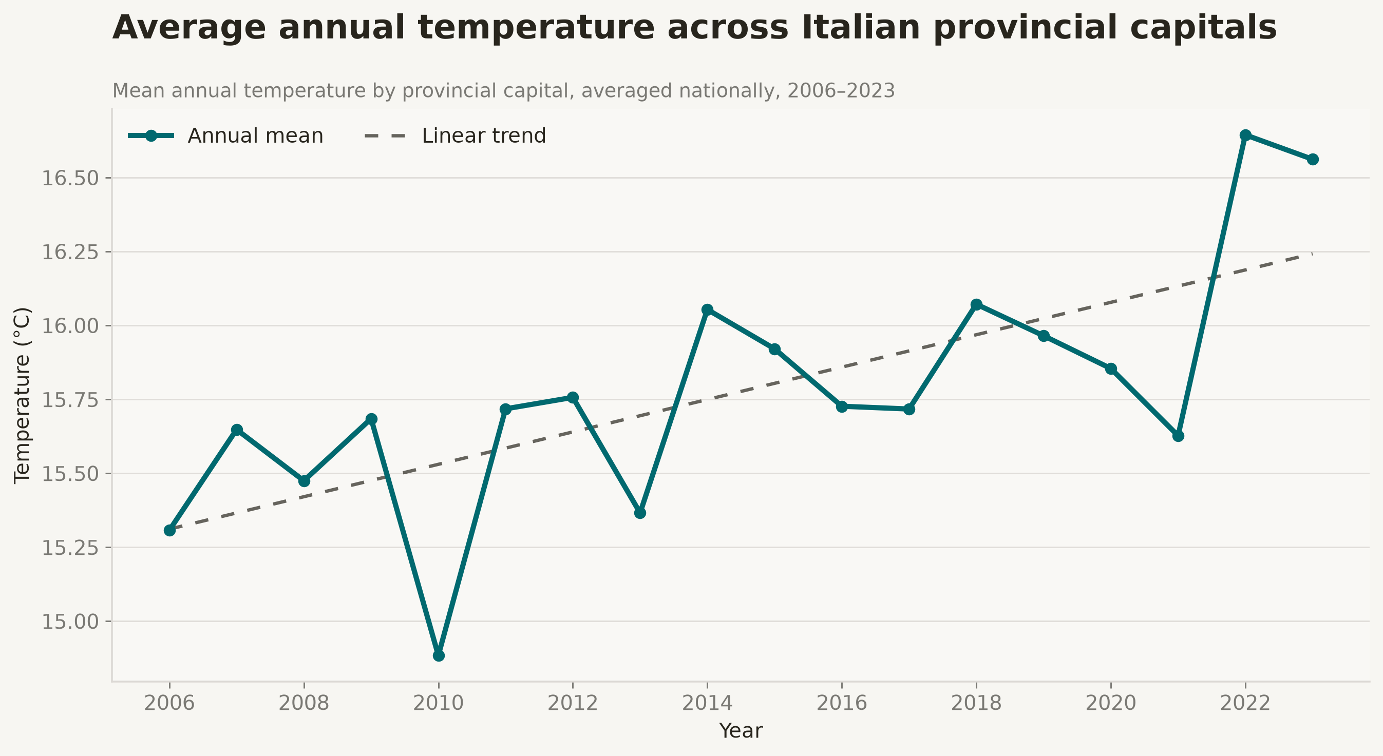
A natural first view is the yearly mean across all provincial capitals. This compresses local variation into a single national summary and makes the direction of change much easier to see.
```{python}
def linear_slope(df, y_col):
    clean = df.dropna(subset=[y_col]).copy()
    x = clean["Year"].to_numpy(dtype=float)
    y = clean[y_col].to_numpy(dtype=float)
    if len(x) < 2:
        return np.nan
    return float(np.polyfit(x, y, 1)[0])


italy_temperature_trend = (
    italy_weather_data.groupby("Year", as_index=False)["Temperature"].mean().dropna()
)

temp_coef = np.polyfit(
    italy_temperature_trend["Year"].to_numpy(dtype=float),
    italy_temperature_trend["Temperature"].to_numpy(dtype=float),
    1,
)
italy_temperature_trend["Trend"] = (
    temp_coef[0] * italy_temperature_trend["Year"] + temp_coef[1]
)

national_temp_slope = linear_slope(italy_temperature_trend, "Temperature")
national_temp_change = national_temp_slope * (2023 - 2006)

national_temp_slope, national_temp_change
```
cross provincial capitals, the fitted warming rate is about **0.055 °C per year**, or roughly **0.9–1.0 °C over the full window**. That does not mean every city warms at exactly the same pace, but it sets the national backdrop for the rest of the analysis.
```{python}
#| label: fig-italy-temperature-trend
#| fig-cap: "Average annual temperature across Italian provincial capitals, 2006–2023."
import numpy as np
import pandas as pd
import matplotlib.pyplot as plt
from matplotlib.ticker import MaxNLocator

def parse_table(sheet_name, value_name):
    df = pd.read_excel(FILE_PATH, sheet_name=sheet_name, header=None)
    years = [int(x) for x in df.iloc[3, 1:19].tolist()]
    data = df.iloc[4:, :19].copy()
    data.columns = ["Province"] + years
    data = data[data["Province"].notna()]
    data["Province"] = data["Province"].astype(str).str.strip()
    data = data[~data["Province"].str.contains(r"Fonte|Totale|Nota|Nelle tavole|^$", regex=True, na=False)]
    long = data.melt(id_vars="Province", var_name="Year", value_name=value_name)
    long["Year"] = pd.to_numeric(long["Year"], errors="coerce")
    long[value_name] = pd.to_numeric(long[value_name].replace("....", np.nan), errors="coerce")
    return long

italy_mean = italy_weather_data.groupby("Year", as_index=False)["Temperature"].mean().dropna()
coef = np.polyfit(italy_mean["Year"], italy_mean["Temperature"], 1)
italy_mean["Trend"] = coef[0] * italy_mean["Year"] + coef[1]

BG = "#f7f6f2"; PANEL = "#f9f8f5"; TEXT = "#28251d"; MUTED = "#7a7974"; GRID = "#dcd9d5"; ACCENT = "#01696f"

plt.rcParams.update({
    "figure.facecolor": BG, "axes.facecolor": PANEL, "axes.edgecolor": GRID, "axes.labelcolor": TEXT,
    "axes.titlecolor": TEXT, "xtick.color": MUTED, "ytick.color": MUTED, "text.color": TEXT,
    "font.size": 11, "axes.titlesize": 18, "axes.titleweight": "bold", "legend.frameon": False
})

fig, ax = plt.subplots(figsize=(10.5, 5.8))
ax.plot(italy_mean["Year"], italy_mean["Temperature"], color=ACCENT, linewidth=2.8, marker="o", markersize=5.5, label="Annual mean", zorder=3)
ax.plot(italy_mean["Year"], italy_mean["Trend"], color=TEXT, linewidth=1.8, linestyle=(0, (4, 4)), alpha=0.7, label="Linear trend", zorder=2)

# Set title with padding and place subtitle below it
ax.set_title("Average annual temperature across Italian provincial capitals", loc="left", pad=38)
ax.text(0, 1.02, "Mean annual temperature by provincial capital, averaged nationally, 2006–2023", transform=ax.transAxes, fontsize=10.5, color=MUTED)

ax.set_xlabel("Year"); ax.set_ylabel("Temperature (°C)")
ax.xaxis.set_major_locator(MaxNLocator(integer=True))
ax.set_xticks(italy_mean["Year"][::2])
ax.grid(axis="y", color=GRID, linewidth=0.8, alpha=0.85)
ax.grid(axis="x", visible=False)
for spine in ["top", "right"]: ax.spines[spine].set_visible(False)
ax.spines["left"].set_color(GRID); ax.spines["bottom"].set_color(GRID)
ax.legend(loc="upper left", ncol=2)

plt.tight_layout()
plt.show()
```
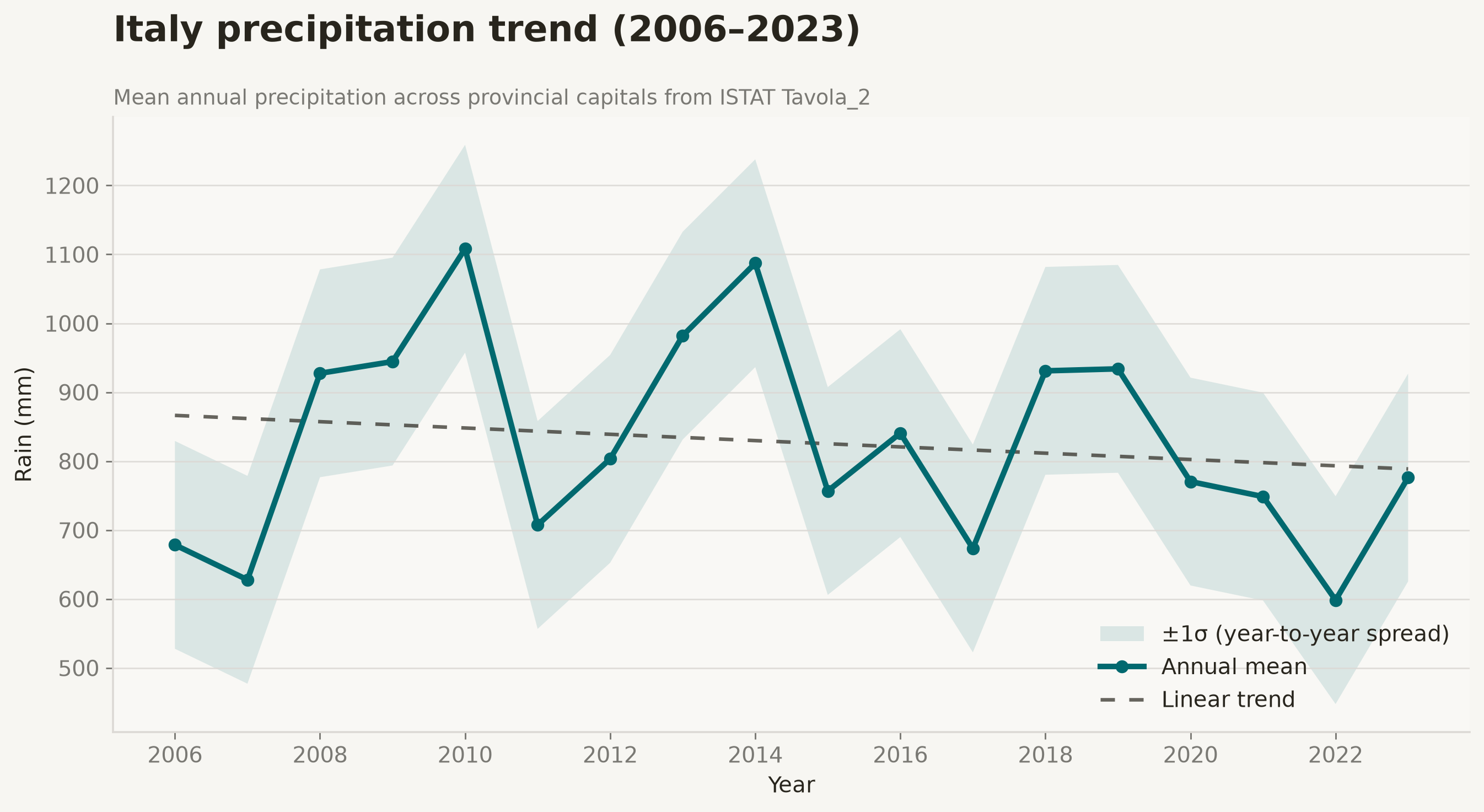
Precipitation is much noisier. The annual mean can still be summarized with a simple line, but the year-to-year swings are much larger than for temperature, so the fitted trend should be read more cautiously. The shaded band in the chart below is a **descriptive spread** — one standard deviation of the yearly national means — added only as a visual guide to how wildly precipitation jumps from year to year. It is *not* a confidence interval or any kind of uncertainty estimate around the trend.
```{python}
italy_precipitation_trend = (
    italy_weather_data.groupby("Year", as_index=False)["Precipitation"]
    .mean()
    .dropna()
)

prec_coef = np.polyfit(
    italy_precipitation_trend["Year"].to_numpy(dtype=float),
    italy_precipitation_trend["Precipitation"].to_numpy(dtype=float),
    1,
)

italy_precipitation_trend["Trend"] = (
    prec_coef[0] * italy_precipitation_trend["Year"] + prec_coef[1]
)

national_prec_slope = linear_slope(
    italy_precipitation_trend,
    "Precipitation"
)
print(f"The overall trend is {round(national_prec_slope, 2)}mm")
```
```{python}
#| label: fig-italy-precipitation-trend
#| fig-cap: "Average annual precipitation across Italian provincial capitals, 2006–2023."
fig, ax = plt.subplots(figsize=(10.5, 5.8))

# Descriptive spread: ±1 standard deviation of the yearly national means.
# This is a visual guide to year-to-year variability, NOT a confidence
# interval or an estimate of uncertainty around the trend line.
prec_std = italy_precipitation_trend["Precipitation"].std()
italy_precipitation_trend["Lower"] = italy_precipitation_trend["Precipitation"] - prec_std
italy_precipitation_trend["Upper"] = italy_precipitation_trend["Precipitation"] + prec_std

# Shaded band
ax.fill_between(italy_precipitation_trend["Year"], italy_precipitation_trend["Lower"], italy_precipitation_trend["Upper"], facecolor=ACCENT, alpha=0.12, linewidth=0, zorder=1, label="±1σ (year-to-year spread)")

# Lines
ax.plot(italy_precipitation_trend["Year"], italy_precipitation_trend["Precipitation"], color=ACCENT, linewidth=2.8, marker="o", markersize=5.5, label="Annual mean", zorder=3)
ax.plot(italy_precipitation_trend["Year"], italy_precipitation_trend["Trend"], color=TEXT, linewidth=1.8, linestyle=(0, (4, 4)), alpha=0.7, label="Linear trend", zorder=2)

# Titles and Subtitles
ax.set_title("Italy precipitation trend (2006–2023)", loc="left", pad=38)
ax.text(0, 1.02, "Mean annual precipitation across provincial capitals from ISTAT Tavola_2", transform=ax.transAxes, fontsize=10.5, color=MUTED)

ax.set_xlabel("Year"); ax.set_ylabel("Rain (mm)")
ax.xaxis.set_major_locator(MaxNLocator(integer=True))
ax.set_xticks(italy_precipitation_trend["Year"][::2])
ax.grid(axis="y", color=GRID, linewidth=0.8, alpha=0.85)
ax.grid(axis="x", visible=False)
for spine in ["top", "right"]: ax.spines[spine].set_visible(False)
ax.spines["left"].set_color(GRID); ax.spines["bottom"].set_color(GRID)
ax.legend(loc="lower right")

plt.tight_layout()
plt.show()
```
# The hottest places
Averaging temperature across the full 2006–2023 period gives a simple "warmest cities" ranking. Unsurprisingly, the leaders cluster in Sicily and the far south.
```{python}
#| label: tbl-hottest-cities
#| tbl-cap: "Five hottest provincial capitals by mean temperature, 2006–2023."
top_hottest = (
    italy_weather_data.groupby("Province", as_index=False)["Temperature"]
    .mean()
    .sort_values("Temperature", ascending=False)
    .head(5)
)

top_hottest
```
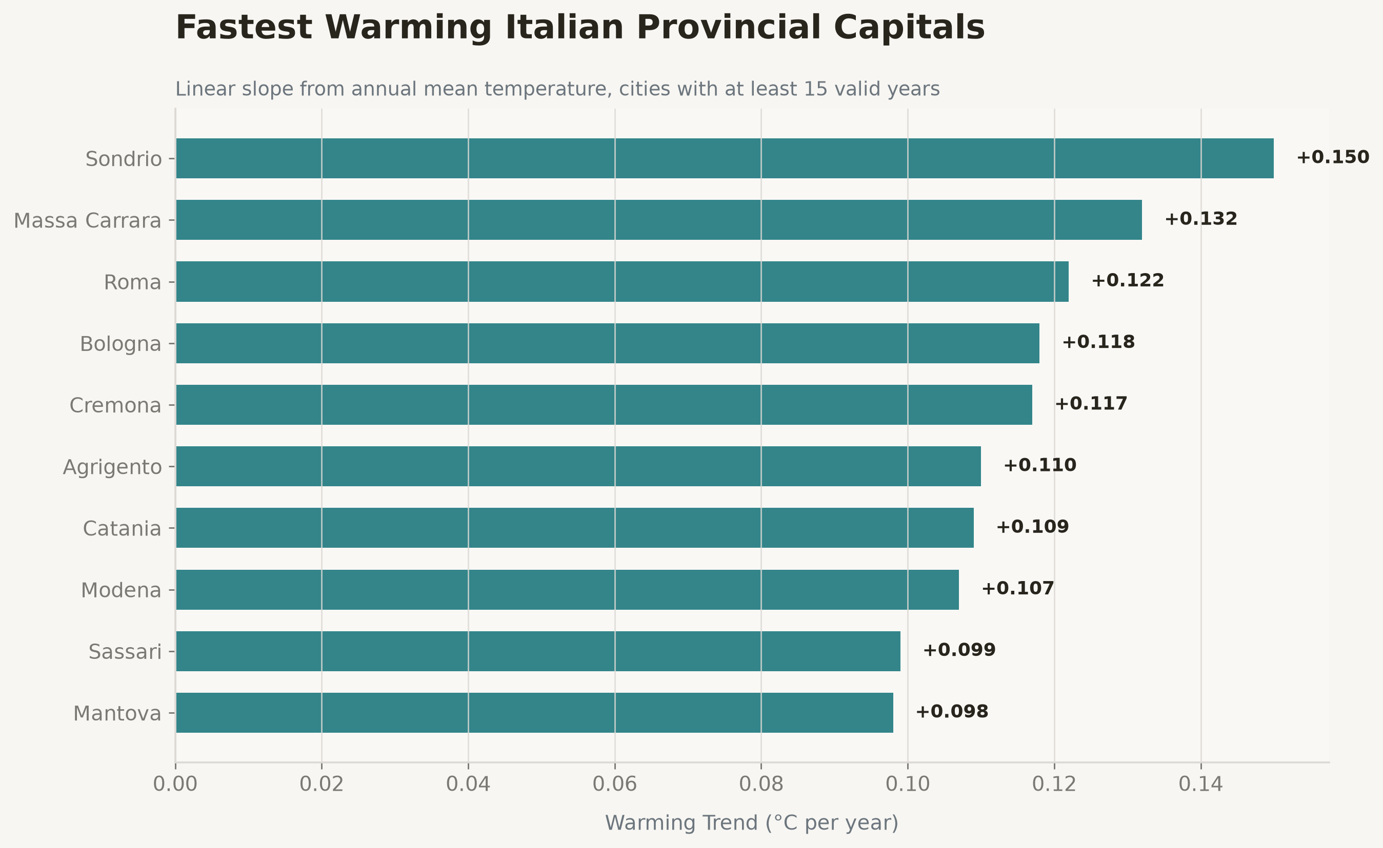
Being hot is not the same as warming quickly. To estimate warming rates, I fit a linear slope for each city after keeping only places with at least 15 valid annual observations, which reduces the influence of patchy reporting histories.
```{python}
def slope_per_city(group, value_col):
    clean = group.dropna(subset=[value_col])
    x = clean["Year"].to_numpy(dtype=float)
    y = clean[value_col].to_numpy(dtype=float)
    if len(x) < 2:
        return np.nan
    return round(float(np.polyfit(x, y, 1)[0]), 3)

warming_base = italy_weather_data.groupby("Province").filter(
    lambda g: g["Temperature"].notna().sum() >= 15
)

warming_rates = (
    warming_base.groupby("Province")
    .apply(lambda g: slope_per_city(g, "Temperature"))
    .rename("Trend (°C/year)")
    .reset_index()
    .sort_values("Trend (°C/year)", ascending=False)
)


warming_rates.head(10)
```
```{python}
#| label: fig-fastest-warming
#| fig-cap: "Fastest warming provincial capitals, filtered to cities with at least 15 valid annual observations."
top_warming = warming_rates.head(10)
fig, ax = plt.subplots(figsize=(10.5, 6.5))

bars = ax.barh(top_warming["Province"][::-1], top_warming["Trend (°C/year)"][::-1], color=ACCENT, alpha=0.8, edgecolor="none", height=0.65)

# Subtitle below title
ax.set_title("Fastest Warming Italian Provincial Capitals", loc="left", pad=38)
ax.text(0, 1.02, "Linear slope from annual mean temperature, cities with at least 15 valid years", transform=ax.transAxes, fontsize=10.5, color=MUTED_HEX)

ax.set_xlabel("Warming Trend (°C per year)", color=MUTED_HEX, fontsize=11, labelpad=10)
for spine in ["top", "right"]: ax.spines[spine].set_visible(False)
ax.spines["left"].set_color(GRID); ax.spines["bottom"].set_color(GRID)
ax.grid(axis="x", linestyle="-", color=GRID, alpha=0.8)
ax.grid(axis="y", visible=False)

for bar in bars:
    width = bar.get_width()
    ax.text(width + 0.003, bar.get_y() + bar.get_height()/2, f"+{width:.3f}", va="center", color=TEXT, fontsize=10, fontweight="bold")

plt.tight_layout()
plt.show()
```
# 2023 anomalies
The long-run series are useful, but the workbook also includes a targeted anomaly table for 2023. `Tavola_3` compares 2023 against the 2006–2015 average and, where available, against the climatological normals for 1981–2010 and 1971–2000.
```{python}
anomaly_sheet = pd.read_excel(FILE_PATH, sheet_name="Tavola_3", header=None)

anomaly_data = anomaly_sheet.iloc[4:114, :7].copy()
anomaly_data.columns = [
    "Province",
    "Diff_2023_vs_2006_2015",
    "Mean_2006_2015",
    "Anom_1981_2010",
    "Clim_1981_2010",
    "Anom_1971_2000",
    "Clim_1971_2000",
]

anomaly_data = anomaly_data[anomaly_data["Province"].notna()]
anomaly_data = anomaly_data[
    ~anomaly_data["Province"].astype(str).str.contains(
        r"Fonte|^\s*$",
        regex=True,
        na=False,
    )
]
anomaly_data["Province"] = anomaly_data["Province"].astype(str).str.strip()

for col in anomaly_data.columns[1:]:
    anomaly_data[col] = pd.to_numeric(
        anomaly_data[col].replace("....", np.nan),
        errors="coerce",
    )

anomaly_data.head()
```
### Understanding the 1981–2010 Baseline
In climate science, an **anomaly** is the difference between the observed temperature and a long-term average called a *climatological normal*. The World Meteorological Organization (WMO) uses 30-year periods to establish these normals.
- **+0.0°C anomaly**: The year was exactly as warm as the 1981–2010 average.
- **Positive anomaly (e.g., +2.66°C)**: The year was warmer than the historical baseline.
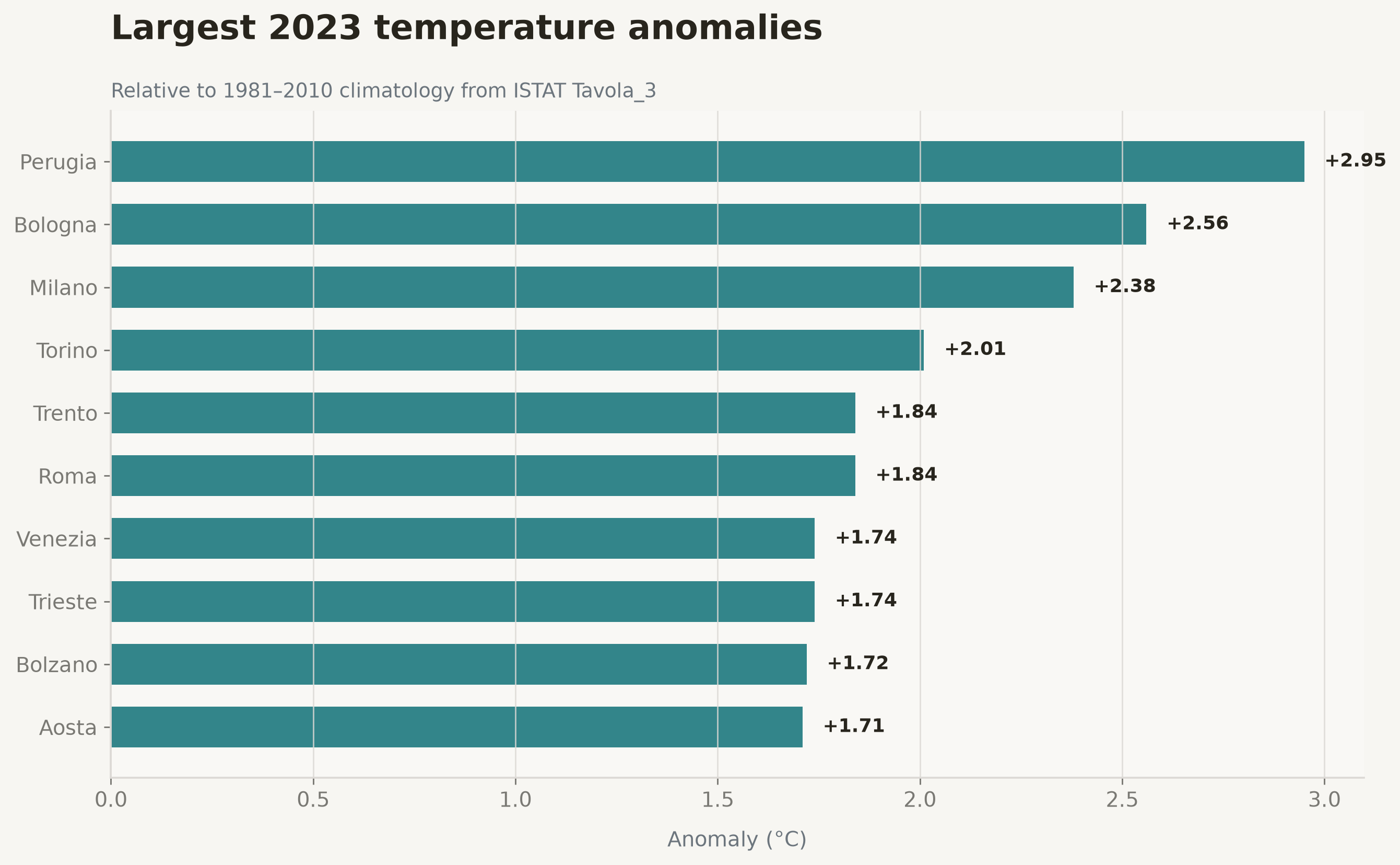
When we see values exceeding +2.0°C in the table below, it indicates that those cities experienced a year significantly hotter than the conditions that characterized the end of the 20th century.
A caveat on coverage: `Tavola_3` does not provide climatological-normal anomalies for every provincial capital. The sheet notes that those reference baselines are calculated only for **regional capitals** with long enough series, and some of the 2023-vs-2006–2015 differences are also missing where the recent series is incomplete. The ranking below is therefore **among places with available climatological comparisons, not all provincial capitals** — it shows which cities stand out within that comparable subset, not an exhaustive list of every warm place in Italy. Within that subset, 2023 stands out particularly strongly in cities such as **Perugia**, **Bologna**, **Milano**, and **Torino**.
```{python}
#| label: tbl-top-anomalies
#| tbl-cap: "Largest 2023 temperature anomalies relative to the 1981–2010 climatology."
top_anomalies = (
    anomaly_data.dropna(subset=["Anom_1981_2010"])
    .sort_values("Anom_1981_2010", ascending=False)
    [["Province", "Anom_1981_2010"]]
    .head(10)
)

top_anomalies
```
```{python}
#| label: fig-2023-anomalies
#| fig-cap: "Largest 2023 temperature anomalies relative to the 1981–2010 climatology."
top_anomalies_plot = anomaly_data.dropna(subset=["Anom_1981_2010"]).sort_values("Anom_1981_2010", ascending=False).head(10)

fig, ax = plt.subplots(figsize=(10.5, 6.5))
bars = ax.barh(top_anomalies_plot["Province"][::-1], top_anomalies_plot["Anom_1981_2010"][::-1], color=ACCENT, alpha=0.8, edgecolor="none", height=0.65)

# Subtitle below title
ax.set_title("Largest 2023 temperature anomalies", loc="left", pad=38)
ax.text(0, 1.02, "Relative to 1981–2010 climatology from ISTAT Tavola_3", transform=ax.transAxes, fontsize=10.5, color=MUTED_HEX)

ax.set_xlabel("Anomaly (°C)", color=MUTED_HEX, fontsize=11, labelpad=10)
for spine in ["top", "right"]: ax.spines[spine].set_visible(False)
ax.spines["left"].set_color(GRID); ax.spines["bottom"].set_color(GRID)
ax.grid(axis="x", linestyle="-", color=GRID, alpha=0.8)
ax.grid(axis="y", visible=False)

for bar in bars:
    width = bar.get_width()
    ax.text(width + 0.05, bar.get_y() + bar.get_height()/2, f"+{width:.2f}", va="center", color=TEXT, fontsize=10, fontweight="bold")

plt.tight_layout()
plt.show()
```
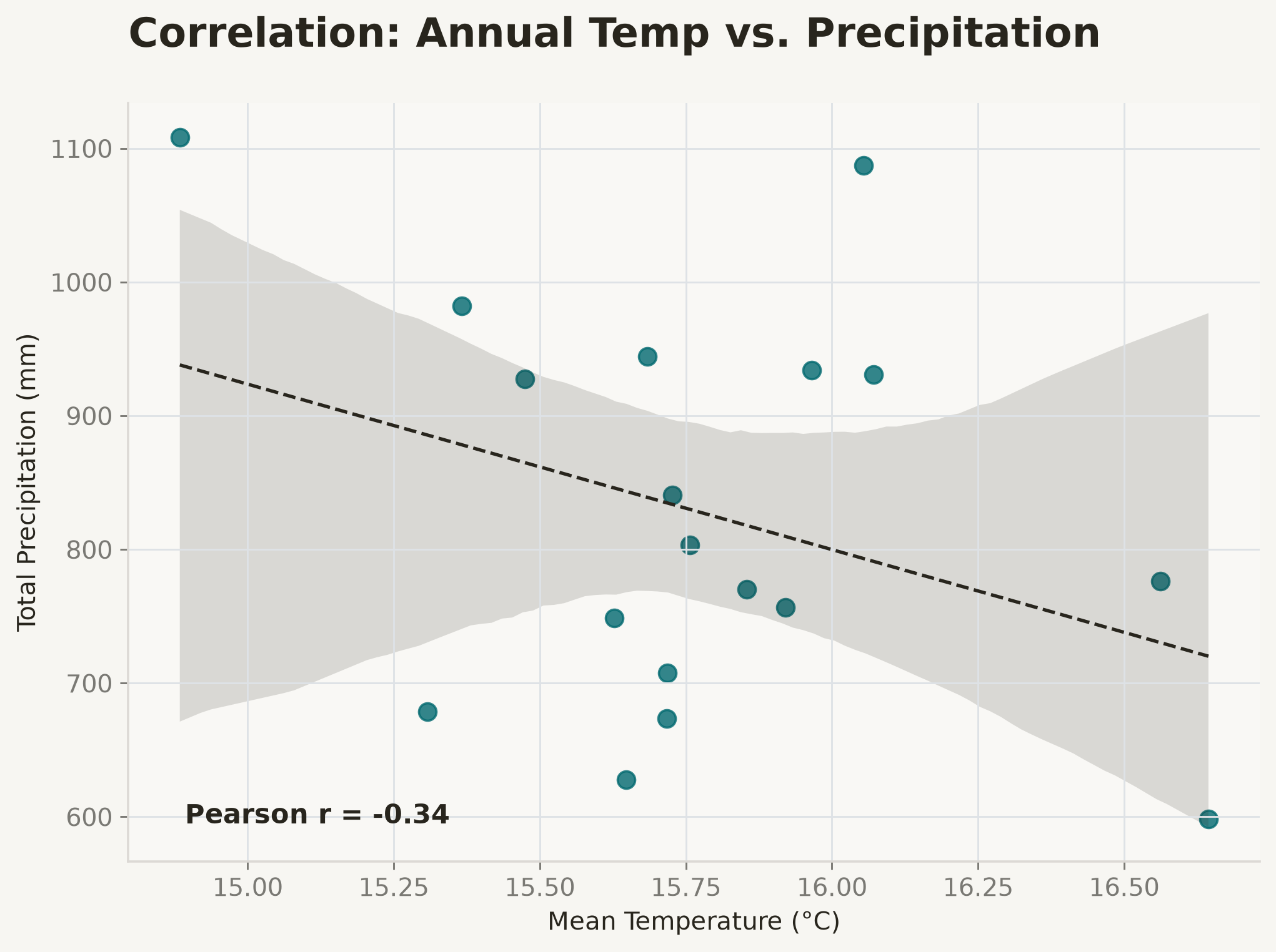
### Correlation: Heat vs. Rainfall
A natural follow-up is whether warmer years also tend to be wetter or drier. Plotting the national annual mean temperature against total precipitation gives a first look at how the two aggregates move together.
```{python}
#| label: fig-2023-heat-vs-rainfall
#| fig-cap: "Correlation: Annual Temp vs. Precipitation."
import seaborn as sns

# Prepare data for correlation
corr_df = italy_temperature_trend[['Year', 'Temperature']].merge(
    italy_precipitation_trend[['Year', 'Precipitation']],
    on='Year'
)

fig, ax = plt.subplots(figsize=(8, 6))
sns.regplot(data=corr_df, x='Temperature', y='Precipitation',
            scatter_kws={'color': ACCENT, 's': 60},
            line_kws={'color': TEXT, 'linestyle': '--', 'linewidth': 1.5}, ax=ax)

ax.set_title("Correlation: Annual Temp vs. Precipitation", loc='left', pad=25)
ax.set_xlabel("Mean Temperature (°C)")
ax.set_ylabel("Total Precipitation (mm)")

# Calculate correlation coefficient
r_val = corr_df['Temperature'].corr(corr_df['Precipitation'])
ax.text(0.05, 0.05, f"Pearson r = {r_val:.2f}", transform=ax.transAxes,
        fontsize=12, fontweight='bold', color=TEXT)

plt.tight_layout()
plt.show()
```
The scatter shows a weak-to-moderate negative association in these annual aggregates: across the 18 years, warmer years have tended to coincide with somewhat lower national precipitation. With a Pearson r of about −0.34 the relationship is real but far from tight — plenty of warm years were not notably dry. This describes only how the two national means co-vary from year to year; it does not say anything about the physical mechanism driving either series, and a single year can move the relationship substantially — the sharp 2022 dip, for instance, reflects the severe drought Italy faced that year and visibly pulls the regression line down.
# Mapping the change
A time-series chart shows *when* temperatures rise. A map shows *where* the warmth sits. To geocode the provincial capitals once, I cache the coordinates locally and reuse them on subsequent renders.
```{python}
#| label: fig-temperature-map
#| fig-cap: "Mean annual temperature by provincial capital for selected years, 2006–2023."
import numpy as np
import pandas as pd
import plotly.express as px
import plotly.io as pio

# Re-defining the parser to ensure data is available
def parse_table(sheet_name, value_name):
    df = pd.read_excel(FILE_PATH, sheet_name=sheet_name, header=None)
    years = [int(x) for x in df.iloc[3, 1:19].tolist()]
    data = df.iloc[4:, :19].copy()
    data.columns = ["Province"] + years
    data = data[data["Province"].notna()]
    data["Province"] = data["Province"].astype(str).str.strip()
    data = data[~data["Province"].str.contains(r"Fonte|Totale|Nota|Nelle tavole|^$", regex=True, na=False)]
    long = data.melt(id_vars="Province", var_name="Year", value_name=value_name)
    long["Year"] = pd.to_numeric(long["Year"], errors="coerce")
    long[value_name] = pd.to_numeric(long[value_name].replace("....", np.nan), errors="coerce")
    return long

# Load data
temp_df = parse_table("Tavola_1", "Temperature")
precip_df = parse_table("Tavola_2", "Precipitation")
italy_weather_data = temp_df.merge(precip_df, on=["Province", "Year"], how="inner")

# A dictionary of coordinates for Italian provincial capitals
city_coords = {
    'Torino': [45.0703, 7.6869], 'Vercelli': [45.3238, 8.4232], 'Novara': [45.4468, 8.6212],
    'Cuneo': [44.3833, 7.5500], 'Asti': [44.9005, 8.2069], 'Alessandria': [44.9129, 8.6154],
    'Biella': [45.5630, 8.0579], 'Verbano-Cusio-Ossola': [45.9220, 8.5516], 'Aosta': [45.7371, 7.3201],
    'Milano': [45.4642, 9.1900], 'Lodi': [45.3139, 9.5032], 'Monza e della Brianza': [45.5845, 9.2744],
    'Bergamo': [45.6983, 9.6773], 'Brescia': [45.5398, 10.2181], 'Pavia': [45.1850, 9.1546],
    'Como': [45.8081, 9.0852], 'Varese': [45.8167, 8.8333], 'Sondrio': [46.1690, 9.8731],
    'Lecco': [45.8559, 9.3977], 'Mantova': [45.1564, 10.7911], 'Cremona': [45.1333, 10.0333],
    'Bolzano': [46.4983, 11.3548], 'Trento': [46.0667, 11.1167], 'Verona': [45.4384, 10.9916],
    'Vicenza': [45.5479, 11.5446], 'Belluno': [46.1408, 12.2161], 'Treviso': [45.6667, 12.2450],
    'Venezia': [45.4408, 12.3155], 'Padova': [45.4064, 11.8768], 'Rovigo': [45.0711, 11.7905],
    'Pordenone': [45.9569, 12.6605], 'Udine': [46.0625, 13.2346], 'Gorizia': [45.9409, 13.6222],
    'Trieste': [45.6495, 13.7768], 'Piacenza': [45.0526, 9.6930], 'Parma': [44.8015, 10.3279],
    'Reggio nell\'Emilia': [44.6982, 10.6312], 'Modena': [44.6471, 10.9252], 'Bologna': [44.4949, 11.3426],
    'Ferrara': [44.8381, 11.6198], 'Ravenna': [44.4183, 12.2035], 'Forlì-Cesena': [44.2227, 12.0409],
    'Rimini': [44.0594, 12.5684], 'Massa Carrara': [44.0375, 10.1417], 'Lucca': [43.8429, 10.5027],
    'Pistoia': [43.9333, 10.9167], 'Firenze': [43.7696, 11.2558], 'Livorno': [43.5485, 10.3106],
    'Pisa': [43.7085, 10.4036], 'Arezzo': [43.4631, 11.8781], 'Siena': [43.3186, 11.3306],
    'Grosseto': [42.7667, 11.1167], 'Prato': [43.8777, 11.1022], 'Perugia': [43.1107, 12.3908],
    'Terni': [42.5639, 12.6427], 'Ancona': [43.6158, 13.5189], 'Pesaro e Urbino': [43.9100, 12.9133],
    'Macerata': [43.3003, 13.4531], 'Ascoli Piceno': [42.8536, 13.5768], 'Fermo': [43.1610, 13.7183],
    'Viterbo': [42.4191, 12.1051], 'Rieti': [42.4000, 12.8667], 'Roma': [41.9028, 12.4964],
    'Latina': [41.4676, 12.9036], 'Frosinone': [41.6394, 13.3411], 'L\'Aquila': [42.3489, 13.3980],
    'Teramo': [42.6589, 13.7044], 'Pescara': [42.4618, 14.2142], 'Chieti': [42.3511, 14.1675],
    'Campobasso': [41.5603, 14.6584], 'Isernia': [41.5947, 14.2342], 'Caserta': [41.0736, 14.3347],
    'Benevento': [41.1297, 14.7821], 'Napoli': [40.8518, 14.2681], 'Avellino': [40.9144, 14.7936],
    'Salerno': [40.6779, 14.7658], 'Foggia': [41.4622, 15.5446], 'Bari': [41.1171, 16.8719],
    'Taranto': [40.4677, 17.2433], 'Brindisi': [40.6321, 17.9361], 'Lecce': [40.3515, 18.1750],
    'Barletta': [41.3197, 16.2768], 'Potenza': [40.6404, 15.8051], 'Matera': [40.6664, 16.6043],
    'Cosenza': [39.2983, 16.2537], 'Catanzaro': [38.9098, 16.5877], 'Reggio di Calabria': [38.1105, 15.6434],
    'Crotone': [39.0808, 17.1273], 'Vibo Valentia': [38.6753, 16.1011], 'Messina': [38.1938, 15.5540],
    'Palermo': [38.1157, 13.3615], 'Trapani': [38.0175, 12.5150], 'Agrigento': [37.3111, 13.5765],
    'Caltanissetta': [37.4903, 14.0622], 'Enna': [37.5671, 14.2750], 'Catania': [37.5079, 15.0830],
    'Ragusa': [36.9269, 14.7231], 'Siracusa': [37.0755, 15.2866], 'Sassari': [40.7259, 8.5615],
    'Nuoro': [40.3231, 9.3303], 'Cagliari': [39.2238, 9.1217], 'Oristano': [39.9056, 8.5911],
    'Carbonia': [39.1671, 8.5222],
    'La Spezia': [44.2384, 9.6912],
    'Andria': [41.2276, 16.2955],
    'Trani': [41.2782, 16.4186],
}

# The workbook uses short province-capital names (e.g. "Verbania", "Monza",
# "Pesaro Urbino", "Forlì") that do not match the longer administrative keys
# in city_coords above. Normalize before lookup so no point disappears
# silently when the dictionary key uses a different spelling.
COORD_NAME_ALIASES = {
    'Verbania': 'Verbano-Cusio-Ossola',
    'Monza': 'Monza e della Brianza',
    'Pesaro Urbino': 'Pesaro e Urbino',
    'Forlì': 'Forlì-Cesena',
}

def lookup_coords(province):
    key = COORD_NAME_ALIASES.get(province, province)
    return city_coords.get(key, [None, None])

# Map coordinates and warn about anything still unmapped so a miss is loud,
# not silent.
italy_weather_data['Lat'] = italy_weather_data['Province'].map(lambda x: lookup_coords(x)[0])
italy_weather_data['Lon'] = italy_weather_data['Province'].map(lambda x: lookup_coords(x)[1])
unmapped = italy_weather_data.loc[italy_weather_data['Lat'].isna(), 'Province'].unique()
if len(unmapped) > 0:
    print(f"Unmapped provinces (no coordinates): {list(unmapped)}")
map_df = italy_weather_data.dropna(subset=['Lat', 'Lon', 'Temperature']).copy()

# Prepare Mapbox map
fig = px.scatter_mapbox(
    map_df,
    lat="Lat", lon="Lon", color="Temperature",
    hover_name="Province", animation_frame="Year",
    title="Evolution of Annual Temperatures in Italy (2006-2023)",
    color_continuous_scale=px.colors.sequential.YlOrRd,
    range_color=[map_df['Temperature'].min(), map_df['Temperature'].max()],
    mapbox_style="open-street-map",
    zoom=4.5, center=dict(lat=42.0, lon=12.5)
)

fig.update_layout(height=700, margin=dict(r=10, t=80, b=40, l=10), paper_bgcolor=globals().get('BG', '#f7f6f2'))
fig
```
A companion view averages each capital across the whole 2006–2023 window, so the persistent north–south gradient — Sicily and the far south glowing warmest, the Alps coolest — is easy to read at a glance.
```{python}
#| label: fig-mean-temperature-map
#| fig-cap: "Mean annual temperature by provincial capital, averaged over 2006–2023."
# Calculate mean per city for the static map
mean_per_city = (
    map_df.groupby("Province", as_index=False)
    .agg(
        Lat=("Lat", "first"),
        Lon=("Lon", "first"),
        Temperature=("Temperature", "mean"),
    )
)

# Create a static Mapbox plot to match the interactive look and feel
fig_static = px.scatter_mapbox(
    mean_per_city,
    lat="Lat",
    lon="Lon",
    color="Temperature",
    hover_name="Province",
    size_max=15,
    color_continuous_scale=px.colors.sequential.YlOrRd,
    range_color=[map_df['Temperature'].min(), map_df['Temperature'].max()],
    mapbox_style="open-street-map",
    zoom=4.5,
    center=dict(lat=42.0, lon=12.5),
    title="<b>Mean temperature by provincial capital (2006–2023)</b><br><span style='font-size:12px; color:#7a7974'>Average temperature across the full series from ISTAT Tavola_1</span>"
)

fig_static.update_layout(
    height=700,
    margin=dict(r=10, t=80, b=40, l=10),
    paper_bgcolor=BG,
    font=dict(color=TEXT)
)

fig_static
```
# Takeaways
The updated workbook makes the national pattern easy to see: Italian provincial capitals show a clear upward temperature trend over 2006–2023, while precipitation is much noisier and less uniform.
A few broad conclusions stand out:
- The average across provincial capitals points to steady warming across the period.
- The warmest cities are concentrated in Sicily and the far south.
- The "fastest warming" ranking depends strongly on data completeness, so filtering sparse series matters.
- The 2023 anomaly table adds important historical context, showing that several cities were not only warm in absolute terms, but unusually warm relative to climatological baselines.
The natural next extension would be to pull in the regional-capital sheets (`Tavola_9` and `Tavola_10`) and the extremes tables (`Tavola_7`, `Tavola_8`, `Tavola_11`–`Tavola_14`) for a second article focused on heat extremes, warm nights, and heavy-rain indicators.
::: {.companion-resources aria-label="Companion resources for the Italian temperatures analysis"}
## Reproduce the analysis
Prefer to run it yourself? The notebook, tidy dataset, and source repository are available so you can inspect the cleaning steps, reuse the data, or extend the charts.
::: {.companion-resources__grid}
::: {.companion-resource}
### Notebook
Run the full analysis locally and reproduce the figures from the article.
[Download `.ipynb`](/downloads/italian_temperatures_2006_2023.ipynb){.btn .btn-primary data-cta-id="italy-temperatures-notebook" download="italian_temperatures_2006_2023.ipynb"}
:::
::: {.companion-resource}
### Tidy dataset
Use the cleaned province-year table with temperature and precipitation columns.
[Download `.csv`](/downloads/italian_temperatures_2006_2023_clean.csv){.btn .btn-outline-primary data-cta-id="italy-temperatures-csv" download="italian_temperatures_2006_2023_clean.csv"}
:::
::: {.companion-resource}
### Source repo
Star or fork the companion GitHub project to build on the analysis.
[View on GitHub](https://github.com/feddernico/temperature-italia){.btn .btn-outline-primary data-cta-id="italy-temperatures-star"}
:::
:::
:::