---
title: "Italian Tourism Occupancy, 1956–2025: From Mass Growth to a New Record"
description: "A reproducible analysis of ISTAT arrivals and nights spent in Italian accommodation establishments, from the long historical series to the post-pandemic recovery."
author: "Federico Viscioletti"
image: "images/italian-tourism-occupancy-analysis.png"
date: "2026-08-10"
lang: en
categories: [data-science, python, tourism, data-visualization]
pillar: data-science-insights
cluster: data-cleaning
pillar-stage: case-study
jupyter: python3
format:
html:
toc: true
code-fold: false
code-tools: true
code-overflow: wrap
embed-resources: false
fig-responsive: true
execute:
warning: false
message: false
echo: true
cache: false
fig-width: 7
fig-height: 4.2
fig-align: center
out-width: 100%
---
<style>
img.cover {
width: 100%;
aspect-ratio: 16 / 9;
object-fit: cover;
object-position: center 45%;
}
.image-credit {
margin-top: -0.5rem;
color: #7a7974;
font-size: 0.8rem;
text-align: right;
}
</style>
<script src="https://cdn.plot.ly/plotly-3.6.0.min.js"></script>
<img src="images/italian-tourism-occupancy-analysis.png" title="Aerial view of blue and white beach umbrellas" class="cover" />
<p class="image-credit">Original photo by <a href="https://unsplash.com/it/@rgaleriacom?utm_source=unsplash&utm_medium=referral&utm_content=creditCopyText">Ricardo Gomez Angel</a> on <a href="https://unsplash.com/it/foto/fotografia-aerea-di-ombrelloni-da-giardino-blu-e-bianchi-hlmuzhcpCkY?utm_source=unsplash&utm_medium=referral&utm_content=creditCopyText">Unsplash</a>.</p>
# Introduction
It is summer, it is hot, and I am thinking about going on holiday. More specifically, I am thinking about the seaside: crowded beaches, full hotels, and the usual question of where everyone is going.
That made me want to look at tourism data. Not just to find out how many people visit Italy, but to understand how tourism has changed over time, which places receive the most visitors, where those visitors come from, and how strongly the whole system still depends on a few summer months.
The data comes from three ISTAT workbooks. One contains the national series from 1956 to 2025; another describes recent tourism by province and guests’ country of residence; the third breaks the data down to Italian municipalities and individual months. They are not exactly designed to tell a story, so the first part of the work is making the different levels and definitions fit together.
The main question I wanted to answer was:
> **How has Italian tourism changed over time, and what does the latest recovery look like once we separate arrivals, nights, destinations, guests’ residence, and seasonality?**
## Quick answers about Italian tourism
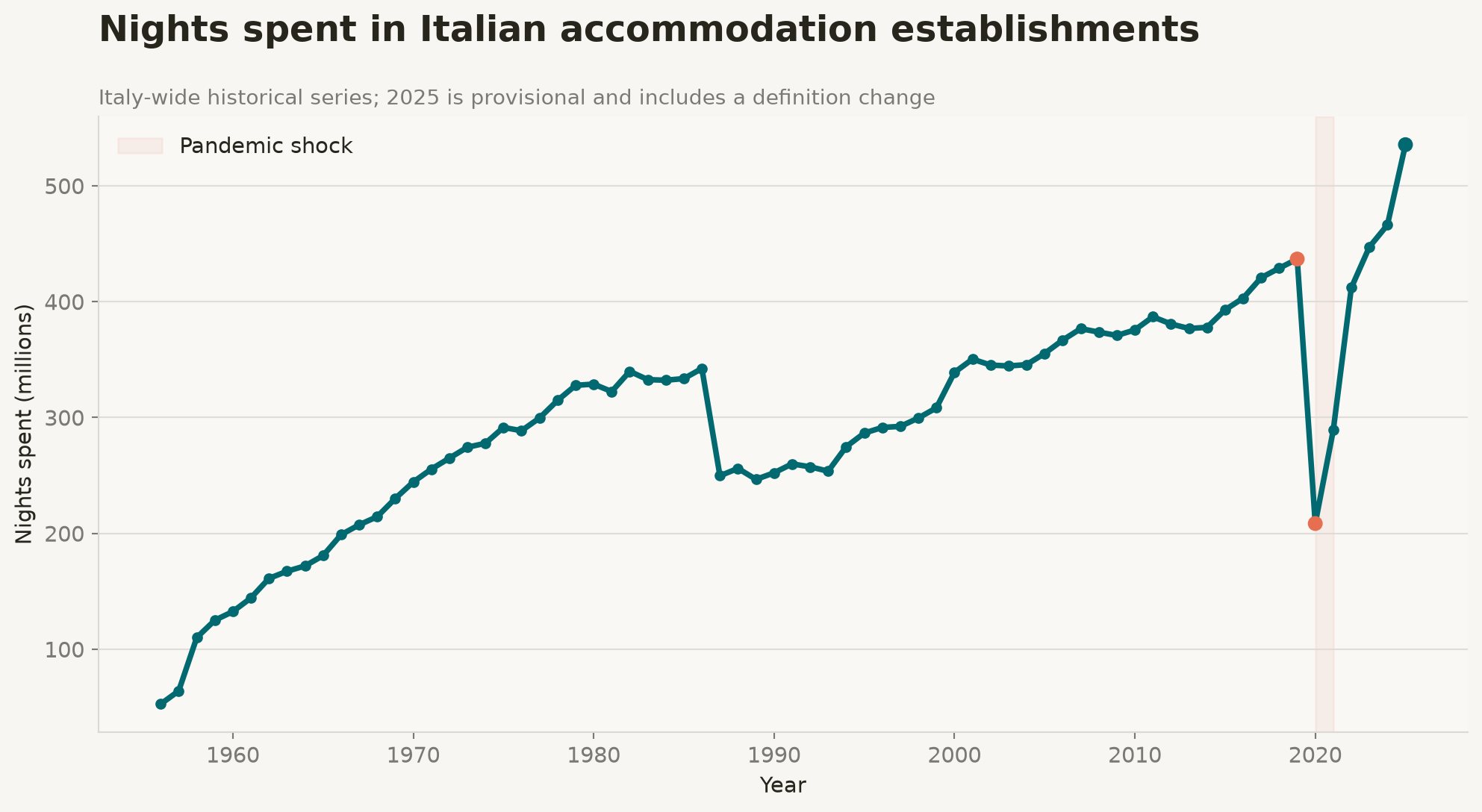
**Did Italian tourism grow over the long run?** Yes. Nights spent in accommodation establishments increased from 52.6 million in 1956 to 436.7 million in 2019. The 2025 provisional figure is higher still, at 535.5 million nights.
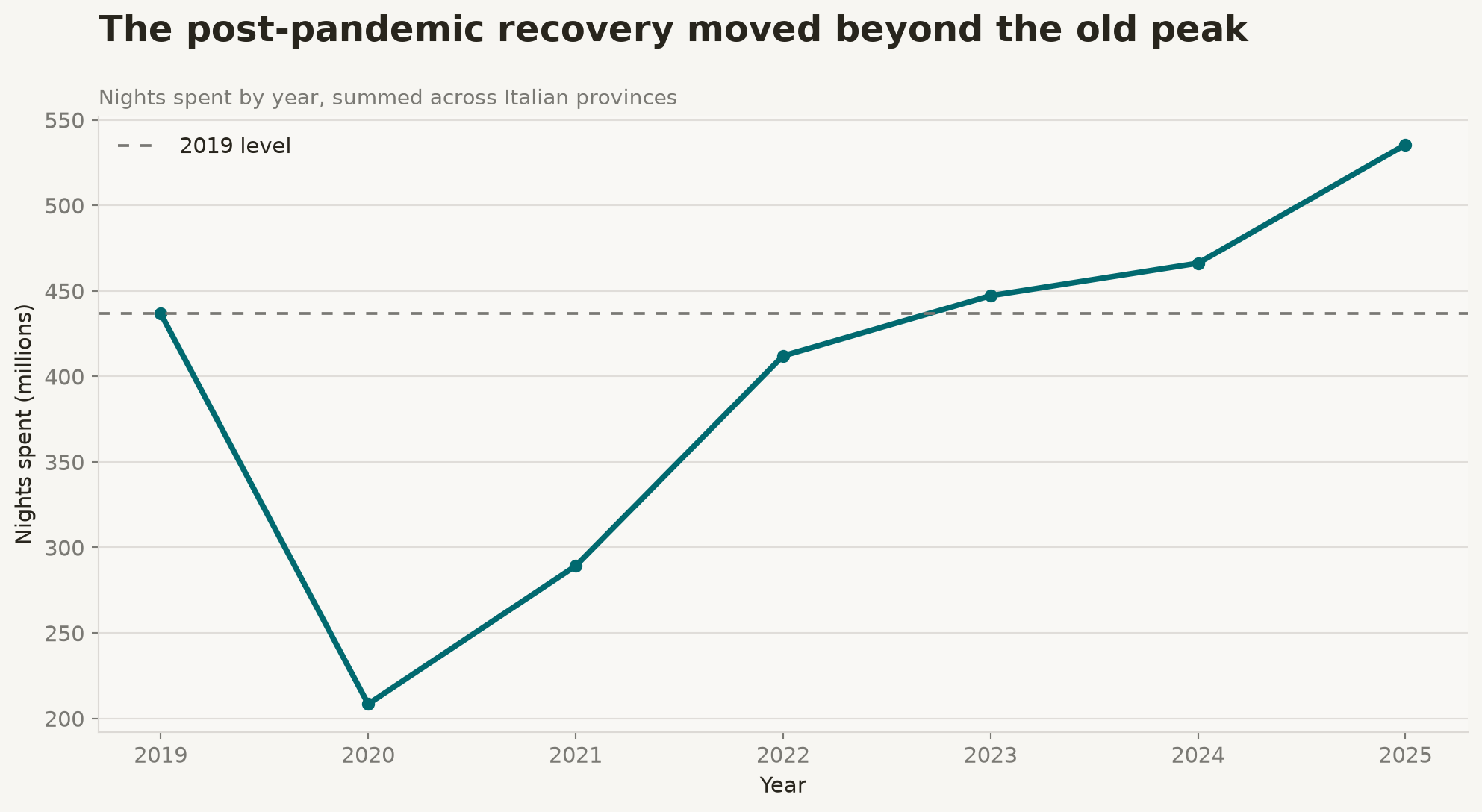
**What did the pandemic do?** Nights spent fell to 208.4 million in 2020 — about 52% below 2019 — before recovering to 466.2 million in 2024 and 535.5 million in 2025.
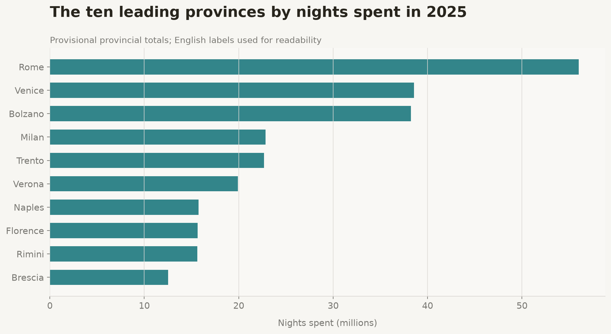
**Where is tourism concentrated?** In 2025, Rome, Venice, Bolzano, Milan, and Trento were the leading provinces by nights spent. The municipal table tells a similar story, with Rome, Milan, Venice, and Florence at the top.
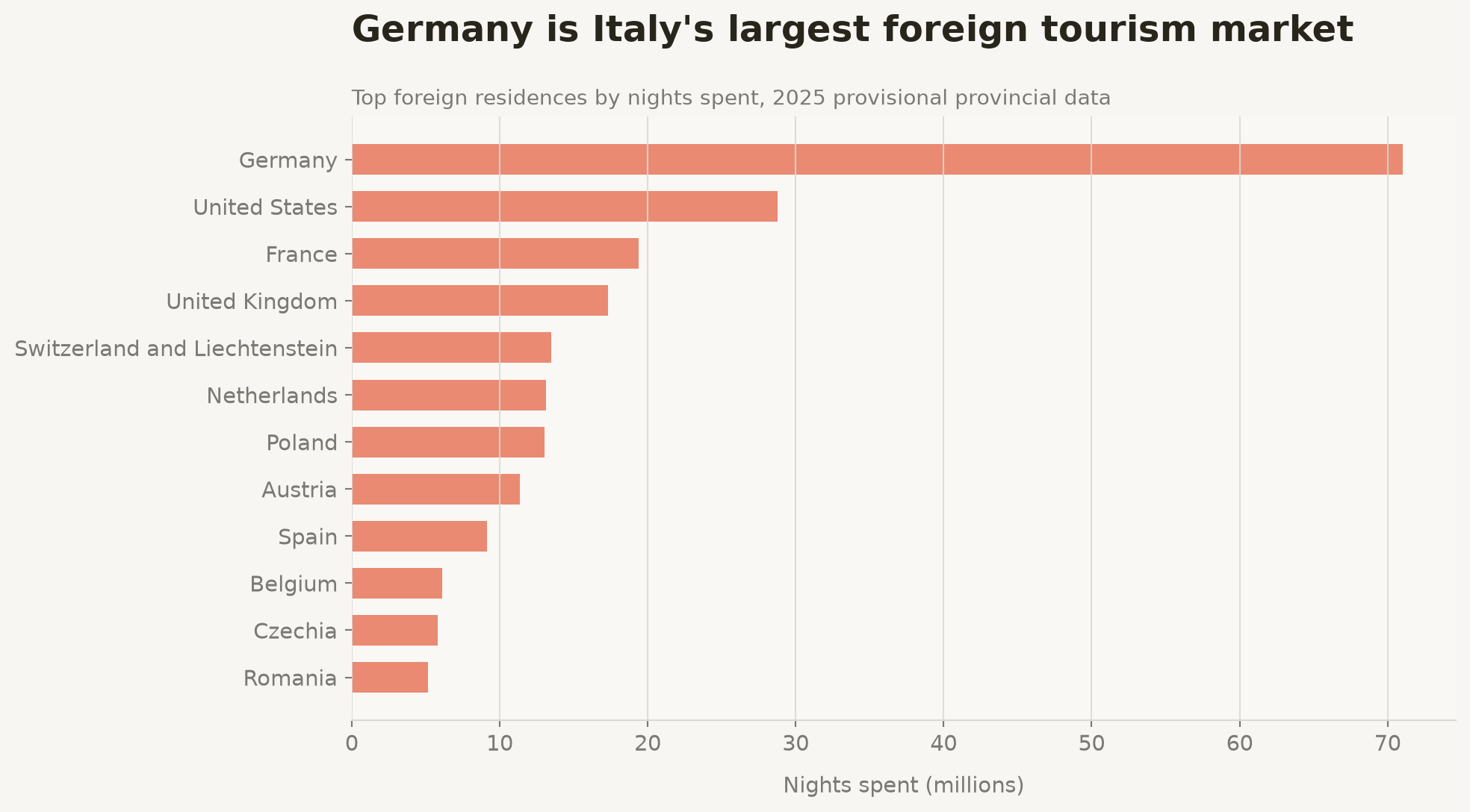
**Who are the international visitors?** In the provincial-by-residence table, Germany is the largest foreign market in 2025, followed by the United States, France, and the United Kingdom.
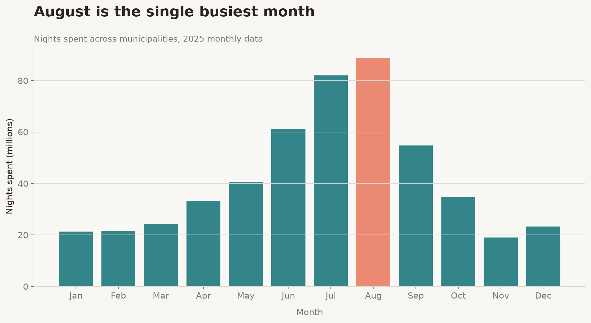
**Is Italian tourism seasonal?** Very much so. August accounts for about 17.6% of the nights recorded in the 2025 monthly municipal file, with July and September also prominent.
The point of this article is not to produce one “tourism score”. It is to show how a few careful reshapes and checks turn official workbooks into a coherent, auditable analysis.
# Loading the ISTAT workbooks
To answer these questions, I used three ISTAT workbooks. They describe Italian tourism at different levels of detail, and each one is useful for a different part of the analysis:
- `1_serie_storica.xlsx`: Italy-wide arrivals and nights spent from 1956 to 2025
- `3_dati_provinciali_per_provenienza.xlsx`: tourism by province and guests’ country of residence from 2019 to 2025
- `2_dati_comunali.xlsx`: annual data by municipality from 2014 to 2025, plus monthly municipal data from 2022 to 2025
The files do not use exactly the same structure or unit of measurement. The historical workbook reports values in thousands, while the provincial and municipal workbooks report individual arrivals and nights. I kept this distinction explicit throughout the analysis rather than converting everything immediately and risking confusion between the series.
Before looking at the results, I needed to clean the files, name the columns clearly, and reshape some of the wider tables into a format that was easier to analyse.
```{python}
#| code-fold: true
#| code-summary: "Show the imports and visual style"
from pathlib import Path

import matplotlib.pyplot as plt
from matplotlib.ticker import FuncFormatter, MaxNLocator
import numpy as np
import pandas as pd
import plotly.graph_objects as go

HISTORICAL_FILE = Path("1_serie_storica.xlsx")
PROVINCIAL_FILE = Path("3_dati_provinciali_per_provenienza.xlsx")
MUNICIPAL_FILE = Path("2_dati_comunali.xlsx")

BG = "#f7f6f2"
PANEL = "#f9f8f5"
TEXT = "#28251d"
MUTED = "#7a7974"
GRID = "#dcd9d5"
TEAL = "#01696f"
CORAL = "#e76f51"

COUNTRY_EN = {
    "Germania": "Germany", "Stati Uniti d'America": "United States",
    "Francia": "France", "Regno Unito": "United Kingdom",
    "Svizzera e Liechtenstein": "Switzerland and Liechtenstein",
    "Paesi Bassi": "Netherlands", "Polonia": "Poland", "Austria": "Austria",
    "Spagna": "Spain", "Belgio": "Belgium", "Canada": "Canada",
    "Australia": "Australia", "Brasile": "Brazil", "Israele": "Israel",
    "India": "India", "Cina": "China", "Giappone": "Japan",
    "Nuova Zelanda": "New Zealand", "Turchia": "Turkey", "Russia": "Russia",
    "Danimarca": "Denmark", "Svezia": "Sweden", "Norvegia": "Norway",
    "Finlandia": "Finland", "Irlanda": "Ireland", "Portogallo": "Portugal",
    "Grecia": "Greece", "Repubblica Ceca": "Czechia", "Romania": "Romania",
}

PROVINCE_EN = {
    "Bolzano-Bozen": "Bolzano", "Venezia": "Venice", "Milano": "Milan",
    "Roma": "Rome", "Firenze": "Florence", "Napoli": "Naples",
    "Torino": "Turin", "Sassari": "Sassari", "Livorno": "Livorno",
    "Brescia": "Brescia", "Verona": "Verona", "Trento": "Trento",
    "Rimini": "Rimini", "Como": "Como", "Siena": "Siena", "Palermo": "Palermo",
    "Udine": "Udine",
}

plt.rcParams.update({
    "figure.facecolor": BG,
    "axes.facecolor": PANEL,
    "axes.edgecolor": GRID,
    "axes.labelcolor": TEXT,
    "axes.titlecolor": TEXT,
    "xtick.color": MUTED,
    "ytick.color": MUTED,
    "text.color": TEXT,
    "font.size": 11,
    "axes.titlesize": 18,
    "axes.titleweight": "bold",
    "legend.frameon": False,
})
pd.options.display.float_format = "{:,.2f}".format
```
## From wide Excel layouts to tidy tables
The first challenge - as always in EDA - was not analysing the data, but reading it properly. The three workbooks were built for publication rather than for analysis: they have different header structures, different levels of detail, and several columns that need to be interpreted before they can be used.
For example, the historical series has two header rows before the actual data begins. The provincial and municipal files instead contain wide blocks of columns split by accommodation type, guest residence, or month. I wrote a small parsing function for each workbook so that these choices were explicit rather than hidden in one long cleaning step.
```{python}
#| code-fold: true
#| code-summary: "Show the workbook parsing functions"
def read_historical(path):
    raw = pd.read_excel(path, header=None).iloc[6:, :19].copy()
    raw.columns = [
        "year", "arrivals_residents", "arrivals_non_residents", "arrivals_total",
        "arrivals_hotels_residents", "arrivals_hotels_non_residents", "arrivals_hotels_total",
        "arrivals_other_residents", "arrivals_other_non_residents", "arrivals_other_total",
        "nights_residents", "nights_non_residents", "nights_total",
        "nights_hotels_residents", "nights_hotels_non_residents", "nights_hotels_total",
        "nights_other_residents", "nights_other_non_residents", "nights_other_total",
    ]
    raw["year"] = pd.to_numeric(raw["year"].astype(str).str.extract(r"(\d{4})")[0], errors="coerce")
    for col in raw.columns[1:]:
        raw[col] = pd.to_numeric(raw[col], errors="coerce")
    return raw.dropna(subset=["year", "arrivals_total", "nights_total"]).astype({"year": int})


def read_provincial(path):
    raw = pd.read_excel(path, header=None).iloc[2:, :21].copy()
    raw.columns = [
        "year", "region_code", "region", "province_code", "province",
        "country_code", "country", *[f"accommodation_{i}" for i in range(14)],
    ]
    data = raw[["year", "region", "province_code", "province", "country_code", "country",
                "accommodation_12", "accommodation_13"]].copy()
    data.columns = ["year", "region", "province_code", "province", "country_code", "country",
                    "arrivals", "nights"]
    data["year"] = pd.to_numeric(data["year"], errors="coerce")
    data["province_code"] = (data["province_code"].astype("string")
                              .str.replace(r"\.0$", "", regex=True)
                              .str.zfill(3))
    data["country_code"] = pd.to_numeric(data["country_code"], errors="coerce")
    data["arrivals"] = pd.to_numeric(data["arrivals"], errors="coerce")
    data["nights"] = pd.to_numeric(data["nights"], errors="coerce")
    data = data.dropna(subset=["year", "country_code", "province", "country", "arrivals", "nights"])
    data["year"] = data["year"].astype(int)
    data[["arrivals", "nights"]] = data[["arrivals", "nights"]].round().astype("Int64")
    return data


def read_municipal_annual(path):
    raw = pd.read_excel(path, sheet_name=0, header=None).iloc[6:, :].copy()
    data = pd.DataFrame({
        "year": pd.to_numeric(raw.iloc[:, 0], errors="coerce"),
        "region": raw.iloc[:, 2].astype("string").str.strip(),
        "province": raw.iloc[:, 4].astype("string").str.strip(),
        "municipality": raw.iloc[:, 5].astype("string").str.strip(),
        "arrivals_residents": pd.to_numeric(raw.iloc[:, 8], errors="coerce"),
        "arrivals_non_residents": pd.to_numeric(raw.iloc[:, 9], errors="coerce"),
        "arrivals": pd.to_numeric(raw.iloc[:, 10], errors="coerce"),
        "nights_residents": pd.to_numeric(raw.iloc[:, 17], errors="coerce"),
        "nights_non_residents": pd.to_numeric(raw.iloc[:, 18], errors="coerce"),
        "nights": pd.to_numeric(raw.iloc[:, 19], errors="coerce"),
    })
    data = data.dropna(subset=["year", "municipality", "arrivals", "nights"]).astype({"year": int})
    count_columns = [column for column in data if column.startswith(("arrivals", "nights"))]
    data[count_columns] = data[count_columns].round().astype("Int64")
    return data


def read_municipal_monthly(path):
    raw = pd.read_excel(path, sheet_name=1, header=None).iloc[4:, :].copy()
    data = pd.DataFrame({
        "year": pd.to_numeric(raw.iloc[:, 0], errors="coerce"),
        "province": raw.iloc[:, 4].astype("string").str.strip(),
        "municipality": raw.iloc[:, 5].astype("string").str.strip(),
        **{f"arrivals_{m:02d}": pd.to_numeric(raw.iloc[:, 8 + m - 1], errors="coerce") for m in range(1, 13)},
        **{f"nights_{m:02d}": pd.to_numeric(raw.iloc[:, 20 + m - 1], errors="coerce") for m in range(1, 13)},
    })
    data = data.dropna(subset=["year", "municipality"]).astype({"year": int})
    count_columns = [column for column in data if column.startswith(("arrivals", "nights"))]
    data[count_columns] = data[count_columns].fillna(0).round().astype("Int64")
    return data


historical = read_historical(HISTORICAL_FILE)
provincial = read_provincial(PROVINCIAL_FILE)
municipal_annual = read_municipal_annual(MUNICIPAL_FILE)
municipal_monthly = read_municipal_monthly(MUNICIPAL_FILE)

historical.agg(start_year=("year", "min"), end_year=("year", "max"), rows=("year", "size"))
```
The main historical table contains 66 reported annual observations from 1956 to 2025. The 2025 row is marked provisional in the source and also introduces a definition change: other privately rented accommodation is included in the tourism-flow data from that year. I therefore use 2024 when comparing the long series with the pre-pandemic period, and label 2025 as provisional wherever it appears.
# The long-term picture: tourism became much bigger
I started with nights spent rather than arrivals. Arrivals tell us how many trips took place, but nights tell us something closer to the actual pressure and scale of tourism: a person staying for one night and a family spending two weeks somewhere should not count in the same way.
The chart below shows the total number of nights spent in Italian accommodation establishments between 1956 and 2025.
```{python}
#| code-fold: true
#| code-summary: "Show the long-run chart code"
history_plot = historical.copy()
history_plot["nights_millions"] = history_plot["nights_total"] / 1_000

fig, ax = plt.subplots(figsize=(10.5, 5.8))
ax.plot(history_plot["year"], history_plot["nights_millions"], color=TEAL, linewidth=2.8, marker="o", markersize=4.5, zorder=2)
ax.scatter([2019, 2020, 2025], history_plot.set_index("year").loc[[2019, 2020, 2025], "nights_millions"],
           color=[CORAL, CORAL, TEAL], s=42, zorder=3)
ax.axvspan(2020, 2021, color=CORAL, alpha=0.08, label="Pandemic shock")
ax.set_title("Nights spent in Italian accommodation establishments", loc="left", pad=38)
ax.text(0, 1.02, "Italy-wide historical series; 2025 is provisional and includes a definition change", transform=ax.transAxes, fontsize=10.5, color=MUTED)
ax.set_xlabel("Year")
ax.set_ylabel("Nights spent (millions)")
ax.grid(axis="y", color=GRID, linewidth=0.8, alpha=0.85)
ax.grid(axis="x", visible=False)
ax.xaxis.set_major_locator(MaxNLocator(integer=True, nbins=9))
ax.legend(loc="upper left")
for spine in ["top", "right"]:
    ax.spines[spine].set_visible(False)
ax.spines["left"].set_color(GRID)
ax.spines["bottom"].set_color(GRID)
plt.tight_layout()
plt.show()
```
The overall direction is clear: Italian tourism became much bigger over the last seventy years. Nights spent rose from 52.6 million in 1956 to 436.7 million in 2019. The provisional figure for 2025 reaches 535.5 million.
But this is not a simple growth story. The series includes changes in how accommodation is classified, a visible discontinuity in the late 1980s, and the sudden collapse caused by the pandemic in 2020.
## What happened around 1987?
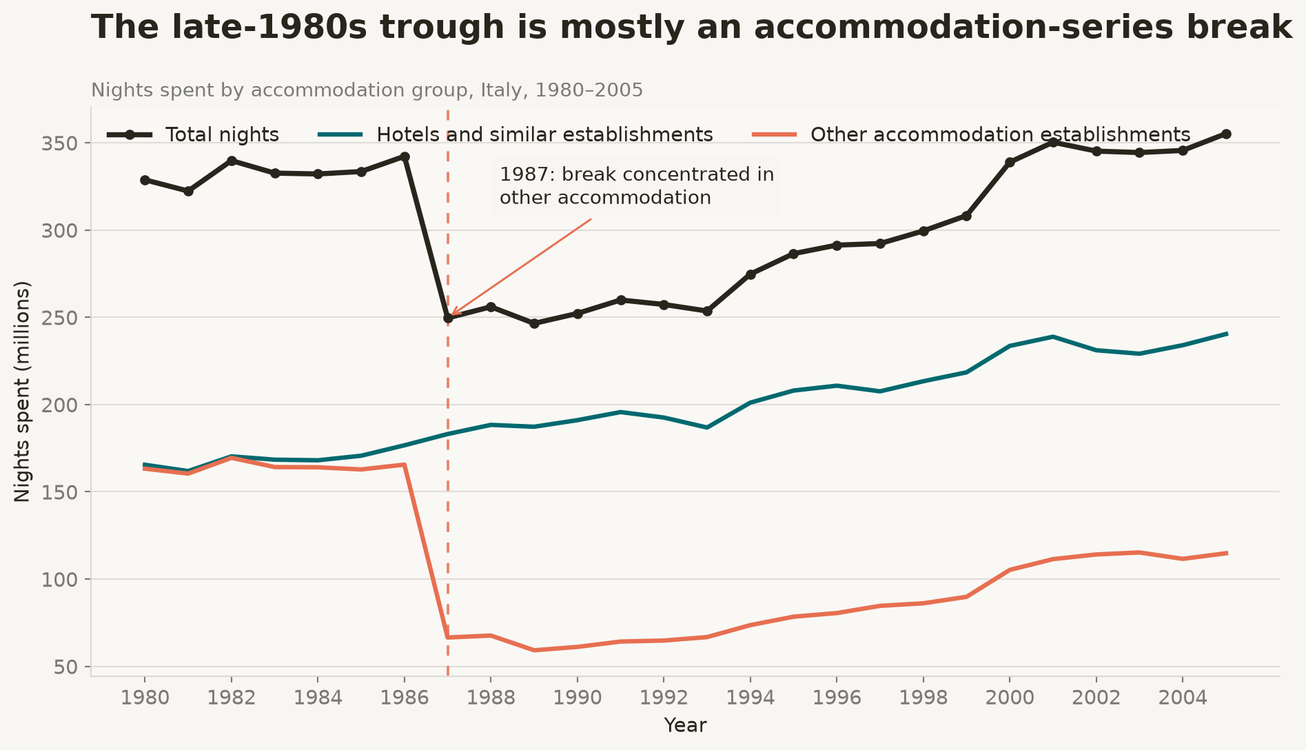
The drop around 1987 immediately caught my attention. Total nights spent fall from 342.3 million in 1986 to 249.7 million in 1987, which looks like a 27.1% collapse in a single year.
But arrivals fall by only 5.3% over the same period. The average stay also declines, from 5.94 to 4.57 nights, but not enough to fully explain such a large fall in total nights. That made me suspect that the break was at least partly about definitions and classification rather than tourists suddenly disappearing.
```{python}
#| code-fold: true
#| code-summary: "Show the late-1980s chart code"
late_eighties = historical.loc[historical["year"].between(1980, 2005)].copy()
for column in ["nights_total", "nights_hotels_total", "nights_other_total"]:
    late_eighties[column + "_millions"] = late_eighties[column] / 1_000

fig, ax = plt.subplots(figsize=(10.5, 5.8))
ax.plot(late_eighties["year"], late_eighties["nights_total_millions"], color=TEXT, linewidth=2.8, marker="o", markersize=4.5, label="Total nights", zorder=3)
ax.plot(late_eighties["year"], late_eighties["nights_hotels_total_millions"], color=TEAL, linewidth=2.4, label="Hotels and similar establishments")
ax.plot(late_eighties["year"], late_eighties["nights_other_total_millions"], color=CORAL, linewidth=2.4, label="Other accommodation establishments")
ax.axvline(1987, color=CORAL, linestyle=(0, (4, 4)), linewidth=1.4, alpha=0.85)
ax.annotate("1987: break concentrated in\nother accommodation", xy=(1987, 249.7), xytext=(1988.2, 315),
            arrowprops=dict(arrowstyle="->", color=CORAL, linewidth=1.1), color=TEXT, fontsize=10.5,
            bbox=dict(boxstyle="round,pad=0.35", facecolor=BG, edgecolor="none", alpha=0.92))
ax.set_title("The late-1980s trough is mostly an accommodation-series break", loc="left", pad=38)
ax.text(0, 1.02, "Nights spent by accommodation group, Italy, 1980–2005", transform=ax.transAxes, fontsize=10.5, color=MUTED)
ax.set_xlabel("Year")
ax.set_ylabel("Nights spent (millions)")
ax.set_xticks(late_eighties["year"][::2])
ax.grid(axis="y", color=GRID, linewidth=0.8, alpha=0.85)
ax.grid(axis="x", visible=False)
for spine in ["top", "right"]:
    ax.spines[spine].set_visible(False)
ax.spines["left"].set_color(GRID)
ax.spines["bottom"].set_color(GRID)
ax.legend(loc="upper left", ncol=3)
plt.tight_layout()
plt.show()
```
The accommodation breakdown makes the issue clearer. Hotel nights increase slightly, from 176.7 million to 183.1 million, while nights in “other accommodation” fall from 165.6 million to 66.5 million.
ISTAT notes a classification change around this point: tourist residences move from extra-hotel to hotel accommodation from 1986. However, that note does not completely explain the fall in the total series, because the total should still include both accommodation groups.
My reading is that the 1987 break combines a genuine reduction in average length of stay with a break in comparability in the accommodation data. I would therefore avoid describing it as a 27% collapse in tourism demand. It is better treated as a point where the historical series becomes less directly comparable.
After 1987, total nights remain around 250–300 million through much of the 1990s and return to the 1986 level only around 2000–2001. Arrivals recover sooner, which suggests that the slower recovery in nights was mainly about shorter stays and changes in the accommodation mix, rather than simply fewer people travelling to Italy.
## The pandemic was a shock, not a new normal
The long historical series shows the scale of the 2020 collapse, but the provincial workbook gives a more detailed view of what happened during the recovery. Unlike the historical series, these data are reported as individual counts rather than thousands.
To calculate national totals from this file, I selected the provincial total rows (`country_code == 0`) and summed them across provinces. I kept individual foreign countries separate, so that aggregate rows would not be counted twice.
```{python}
prov_total = (
    provincial[provincial["country_code"].eq(0)]
    .groupby("year", as_index=False)[["arrivals", "nights"]].sum()
)
prov_total["average_stay"] = prov_total["nights"] / prov_total["arrivals"]
prov_total["nights_millions"] = prov_total["nights"] / 1_000_000
prov_total["change_vs_2019"] = prov_total["nights"] / prov_total.loc[prov_total.year.eq(2019), "nights"].iloc[0] - 1
prov_total
```
```{python}
#| code-fold: true
#| code-summary: "Show the recovery chart code"
fig, ax = plt.subplots(figsize=(10.5, 5.8))
ax.plot(prov_total["year"], prov_total["nights_millions"], color=TEAL, linewidth=2.8, marker="o", markersize=5.5)
ax.axhline(prov_total.loc[prov_total.year.eq(2019), "nights_millions"].iloc[0], color=MUTED, linestyle=(0, (4, 4)), linewidth=1.4, label="2019 level")
ax.set_title("The post-pandemic recovery moved beyond the old peak", loc="left", pad=38)
ax.text(0, 1.02, "Nights spent by year, summed across Italian provinces", transform=ax.transAxes, fontsize=10.5, color=MUTED)
ax.set_xlabel("Year")
ax.set_ylabel("Nights spent (millions)")
ax.set_xticks(prov_total["year"])
ax.grid(axis="y", color=GRID, linewidth=0.8, alpha=0.85)
ax.grid(axis="x", visible=False)
ax.legend(loc="upper left")
for spine in ["top", "right"]:
    ax.spines[spine].set_visible(False)
ax.spines["left"].set_color(GRID)
ax.spines["bottom"].set_color(GRID)
plt.tight_layout()
plt.show()
```
The recovery also changed the mix of visitors. Foreign residents accounted for about 50.5% of nights in 2019, fell to 31.4% in 2020, and reached 54.5% in 2024 in the historical series. That makes the rebound look less like a simple return of domestic demand and more like the reopening of Italy's international tourism circuit.
# Where the nights are spent
The provincial totals show a concentrated geography: a small group of destinations captures a large share of the national market. The ranking is not just a ranking of large cities. It also includes resort systems and provinces whose accommodation capacity serves a whole landscape — the Dolomites, the Venetian lagoon, Lake Garda, or the Roman metropolitan area.
```{python}
latest_provinces = (
    provincial.query("year == 2025 and country_code == 0")
    .nlargest(10, "nights")[["province", "nights", "arrivals"]]
    .assign(nights_millions=lambda d: d["nights"] / 1_000_000)
)
latest_provinces["province_en"] = (
    latest_provinces["province"].astype("string").str.strip().str.title()
    .map(PROVINCE_EN).fillna(latest_provinces["province"])
)
latest_provinces = latest_provinces.drop(columns="province")
latest_provinces = latest_provinces.rename(columns={"province_en": "province"})
latest_provinces = latest_provinces[["province"] + [col for col in latest_provinces.columns if col != "province"]]
latest_provinces
```
```{python}
fig, ax = plt.subplots(figsize=(10.5, 5.8))
plot_data = latest_provinces.sort_values("nights_millions")
ax.barh(plot_data["province"], plot_data["nights_millions"], color=TEAL, alpha=0.8, edgecolor="none", height=0.65)
ax.set_title("The ten leading provinces by nights spent in 2025", loc="left", pad=38)
ax.text(0, 1.02, "Provisional provincial totals; English labels used for readability", transform=ax.transAxes, fontsize=10.5, color=MUTED)
ax.set_xlabel("Nights spent (millions)", color=MUTED, fontsize=11, labelpad=10)
ax.grid(axis="x", color=GRID, linewidth=0.8, alpha=0.85)
ax.grid(axis="y", visible=False)
for spine in ["top", "right", "left"]:
    ax.spines[spine].set_visible(False)
ax.spines["bottom"].set_color(GRID)
plt.tight_layout()
plt.show()
```
Rome led the 2025 provincial table with 56.0 million nights, followed by Venice and Bolzano. The municipal table provides a useful cross-check: it puts Rome, Milan, Venice, and Florence at the top when the analysis is performed at destination-municipality level. The small difference between the provincial and municipal totals is a reminder that official tables can have different coverage and disclosure rules; they should be compared as complementary views, not mechanically stacked together.
# Who is visiting Italy?
The residence table is especially useful because it turns “international tourism” into a set of visible flows. The chart below excludes `TOTALE`, Italian regions, and other aggregate codes, then ranks individual foreign residences by nights spent in 2025.
```{python}
foreign_2025 = provincial.query("year == 2025 and country_code.between(1, 887)")
top_markets = (
    foreign_2025.groupby("country", as_index=False)[["arrivals", "nights"]].sum()
    .nlargest(12, "nights")
    .assign(nights_millions=lambda d: d["nights"] / 1_000_000)
)
top_markets["country_en"] = top_markets["country"].map(COUNTRY_EN).fillna(top_markets["country"])
top_markets = top_markets.drop(columns="country")
top_markets = top_markets.rename(columns={"country_en": "country"})
top_markets = top_markets[["country"] + [col for col in top_markets.columns if col != "country"]]
top_markets
```
```{python}
fig, ax = plt.subplots(figsize=(10.5, 5.8))
plot_data = top_markets.sort_values("nights_millions")
ax.barh(plot_data["country"], plot_data["nights_millions"], color=CORAL, alpha=0.8, edgecolor="none", height=0.65)
ax.set_title("Germany is Italy's largest foreign tourism market", loc="left", pad=38)
ax.text(0, 1.02, "Top foreign residences by nights spent, 2025 provisional provincial data", transform=ax.transAxes, fontsize=10.5, color=MUTED)
ax.set_xlabel("Nights spent (millions)", color=MUTED, fontsize=11, labelpad=10)
ax.grid(axis="x", color=GRID, linewidth=0.8, alpha=0.85)
ax.grid(axis="y", visible=False)
for spine in ["top", "right", "left"]:
    ax.spines[spine].set_visible(False)
ax.spines["bottom"].set_color(GRID)
plt.tight_layout()
plt.show()
```
Germany contributed 71.0 million nights in the 2025 provincial file, more than twice the United States total. The ranking is a useful descriptive view of demand, not a measure of the value or profitability of each market: average stay, accommodation type, spending, and geography differ across countries.
# August still owns the calendar
Annual totals hide the operational rhythm of tourism. The monthly municipal file covers 2022–2025; filtering it to 2025 and summing the twelve monthly columns shows how concentrated demand is in the summer.
```{python}
monthly_2025 = municipal_monthly.query("year == 2025").copy()
monthly_nights = pd.Series({
    month: monthly_2025[f"nights_{month:02d}"].sum()
    for month in range(1, 13)
})
monthly_nights.index = ["Jan", "Feb", "Mar", "Apr", "May", "Jun", "Jul", "Aug", "Sep", "Oct", "Nov", "Dec"]
monthly_nights = monthly_nights / 1_000_000
monthly_nights.to_frame("nights_millions")
```
```{python}
#| code-fold: true
#| code-summary: "Show the monthly seasonality chart code"
fig, ax = plt.subplots(figsize=(10.5, 5.8))
colors = [CORAL if month == "Aug" else TEAL for month in monthly_nights.index]
ax.bar(monthly_nights.index, monthly_nights, color=colors, alpha=0.8, edgecolor="none")
ax.set_title("August is the single busiest month", loc="left", pad=38)
ax.text(0, 1.02, "Nights spent across municipalities, 2025 monthly data", transform=ax.transAxes, fontsize=10.5, color=MUTED)
ax.set_xlabel("Month", color=MUTED, fontsize=11, labelpad=10)
ax.set_ylabel("Nights spent (millions)")
ax.grid(axis="y", color=GRID, linewidth=0.8, alpha=0.85)
ax.grid(axis="x", visible=False)
for spine in ["top", "right"]:
    ax.spines[spine].set_visible(False)
ax.spines["left"].set_color(GRID)
ax.spines["bottom"].set_color(GRID)
plt.tight_layout()
plt.show()
```
August accounts for roughly 17.6% of the nights in the 2025 monthly municipal file. July and September add another large block around it, which matters for transport, staffing, water use, housing pressure, and the environmental footprint of destinations. A national annual total is therefore only the beginning of the planning question.
# Reading the flows: from residence to destination
The previous charts rank places and markets independently. The two views below keep the relationship between them visible. First, a Sankey diagram shows how the leading foreign residences connect to the leading Italian provinces in 2025. The colours follow the article palette: coral identifies origin markets and teal identifies Italian destinations.
```{python}
#| code-fold: true
#| code-summary: "Show the Sankey chart code"
SANKey_YEAR = 2025
TOP_COUNTRIES = 12
TOP_PROVINCES = 15
MIN_PRESENCES = 1_000

flow_data = provincial.query(
    "year == @SANKey_YEAR and country_code.between(1, 887) and nights >= @MIN_PRESENCES"
).copy()
flow_data["country"] = flow_data["country"].astype(str).str.strip()
flow_data["province"] = flow_data["province"].astype(str).str.strip().str.title()
flow_data = (
    flow_data.groupby(["country_code", "country", "province"], as_index=False)
    .agg(arrivals=("arrivals", "sum"), nights=("nights", "sum"))
)

top_countries_flow = (
    flow_data.groupby(["country_code", "country"], as_index=False)["nights"]
    .sum()
    .nlargest(TOP_COUNTRIES, "nights")
)
top_provinces_flow = (
    flow_data.groupby("province", as_index=False)["nights"]
    .sum()
    .nlargest(TOP_PROVINCES, "nights")
)
flow_data = flow_data.merge(top_countries_flow[["country_code", "country"]], on=["country_code", "country"])
flow_data = flow_data.merge(top_provinces_flow[["province"]], on="province")

province_coordinates = {
    "Bolzano-Bozen": (46.4983, 11.3548), "Verona": (45.4385, 10.9938),
    "Livorno": (43.5443, 10.3262), "Brescia": (45.5356, 10.2147),
    "Udine": (46.0711, 13.2346),
    "Torino": (45.0703, 7.6869),
    "Venezia": (45.4333, 12.3500), "Trento": (46.0667, 11.1333),
    "Rimini": (44.0667, 12.5667), "Sassari": (40.7167, 8.5667),
    "Como": (45.8000, 9.0833), "Siena": (43.3167, 11.3000),
    "Palermo": (38.1166, 13.3636), "Milano": (45.4643, 9.1895),
    "Napoli": (40.8522, 14.2681), "Roma": (41.9000, 12.4833),
    "Firenze": (43.7667, 11.2500),
}

province_totals_flow = flow_data.groupby("province", as_index=False)["nights"].sum()
missing_provinces = sorted(set(province_totals_flow["province"]) - set(province_coordinates))
if missing_provinces:
    raise ValueError(f"Missing coordinates for Sankey provinces: {missing_provinces}")

country_totals_flow = (
    flow_data.groupby(["country_code", "country"], as_index=False)["nights"]
    .sum()
    .sort_values("nights", ascending=False)
    .reset_index(drop=True)
)
province_totals_flow = province_totals_flow.assign(
    latitude=province_totals_flow["province"].map(lambda p: province_coordinates[p][0])
).sort_values(["latitude", "province"], ascending=[False, True]).reset_index(drop=True)

ISO2_BY_NUMERIC = {
    1: "FR", 3: "NL", 4: "DE", 6: "GB", 7: "IE", 8: "DK", 9: "GR", 10: "PT", 11: "ES",
    17: "BE", 18: "LU", 24: "IS", 28: "NO", 30: "SE", 32: "FI", 36: "CH", 38: "AT",
    52: "TR", 55: "LT", 60: "PL", 61: "CZ", 63: "SK", 64: "HU", 66: "RO", 68: "BG",
    72: "UA", 75: "RU", 400: "US", 404: "CA", 508: "BR", 624: "IL", 664: "IN",
    720: "CN", 732: "JP", 800: "AU", 804: "NZ",
}

def flag(iso2):
    if not iso2 or len(iso2) != 2:
        return "🌍"
    return "".join(chr(127397 + ord(c)) for c in iso2.upper())


country_nodes = [
    f"{flag(ISO2_BY_NUMERIC.get(int(row.country_code)))} {COUNTRY_EN.get(row.country, row.country)}"
    for row in country_totals_flow.itertuples(index=False)
]
province_nodes = [f"🇮🇹 {PROVINCE_EN.get(p, p)}" for p in province_totals_flow["province"]]
labels = country_nodes + province_nodes
country_y = np.linspace(0.03, 0.97, len(country_nodes))
province_y = np.linspace(0.03, 0.97, len(province_nodes))
node_x = [0.01] * len(country_nodes) + [0.99] * len(province_nodes)
node_y = country_y.tolist() + province_y.tolist()

country_index = {
    (int(row.country_code), row.country): i
    for i, row in enumerate(country_totals_flow.itertuples(index=False))
}
province_index = {
    p: len(country_nodes) + i
    for i, p in enumerate(province_totals_flow["province"])
}
sources = [country_index[(int(r.country_code), r.country)] for r in flow_data.itertuples(index=False)]
targets = [province_index[r.province] for r in flow_data.itertuples(index=False)]
link_codes = flow_data["country_code"].astype(int).tolist()

default_links = ["rgba(1, 105, 111, 0.28)"] * len(flow_data)
default_nodes = (["rgba(231, 111, 81, 0.88)"] * len(country_nodes)
                 + ["rgba(1, 105, 111, 0.78)"] * len(province_nodes))
hover = [
    f"<b>{flag(ISO2_BY_NUMERIC.get(int(r.country_code)))} {COUNTRY_EN.get(r.country, r.country)} → 🇮🇹 {PROVINCE_EN.get(r.province, r.province)}</b><br>"
    f"Nights spent: {r.nights:,.0f}<br>Arrivals: {r.arrivals:,.0f}<br>"
    f"Average stay: {r.nights / r.arrivals:.2f} nights"
    if r.arrivals else f"<b>{COUNTRY_EN.get(r.country, r.country)} → {PROVINCE_EN.get(r.province, r.province)}</b><br>Nights spent: {r.nights:,.0f}"
    for r in flow_data.itertuples(index=False)
]

sankey_fig = go.Figure(go.Sankey(
    arrangement="snap",
    node=dict(
        pad=24, thickness=18, x=node_x, y=node_y,
        line=dict(color="#ffffff", width=0.8), label=labels, color=default_nodes,
        hovertemplate="%{label}<br>%{value:,.0f} nights spent<extra></extra>",
    ),
    link=dict(
        source=sources, target=targets, value=flow_data["nights"], color=default_links,
        customdata=hover, hovertemplate="%{customdata}<extra></extra>",
    ),
))

sankey_buttons = [dict(
    label="All countries", method="restyle",
    args=[{"link.color": [default_links], "node.color": [default_nodes], "node.label": [labels]}],
)]
for row in country_totals_flow.itertuples(index=False):
    selected = int(row.country_code)
    selected_provinces = set(flow_data.loc[flow_data["country_code"].eq(selected), "province"])
    selected_links = [
        "rgba(231, 111, 81, 0.90)" if code == selected else "rgba(108, 117, 125, 0.035)"
        for code in link_codes
    ]
    selected_nodes = [
        "rgba(231, 111, 81, 0.95)" if int(code) == selected else "rgba(108, 117, 125, 0)"
        for code in country_totals_flow["country_code"]
    ] + [
        "rgba(1, 105, 111, 0.95)" if province in selected_provinces else "rgba(108, 117, 125, 0)"
        for province in province_totals_flow["province"]
    ]
    selected_labels = [
        label if int(code) == selected else ""
        for label, code in zip(country_nodes, country_totals_flow["country_code"])
    ] + [
        label if province in selected_provinces else ""
        for label, province in zip(province_nodes, province_totals_flow["province"])
    ]
    sankey_buttons.append(dict(
        label=f"{flag(ISO2_BY_NUMERIC.get(selected))} {COUNTRY_EN.get(row.country, row.country)}", method="restyle",
        args=[{"link.color": [selected_links], "node.color": [selected_nodes], "node.label": [selected_labels]}],
    ))

sankey_fig.update_layout(
    title=dict(text=f"From foreign residences to Italian provinces: tourism flows {SANKey_YEAR}", x=0.02, xanchor="left"),
    font=dict(family="Arial, sans-serif", size=13, color=TEXT),
    paper_bgcolor=BG, plot_bgcolor=BG, margin=dict(l=20, r=20, t=145, b=20), height=900,
    updatemenus=[dict(
        buttons=sankey_buttons, direction="down", x=0.02, y=1.16, xanchor="left", yanchor="top",
        bgcolor=PANEL, bordercolor=GRID, borderwidth=1, font=dict(size=13),
    )],
    annotations=[dict(
        text="Select a country to highlight its destination flows.", x=0.02, y=1.08,
        xref="paper", yref="paper", showarrow=False, xanchor="left", font=dict(size=12, color=MUTED),
    )],
)
sankey_fig
```
The Sankey is deliberately filtered to the leading markets, destinations, and links above a minimum size. That keeps the visual legible while preserving the same country-to-province logic as the original standalone analysis. Select a country from the dropdown to isolate its network.
## Following the flows across years
The second view animates the same idea over time. To keep the article self-contained and reproducible, it uses a small local coordinate table for the leading foreign markets and province capitals rather than downloading geographic files at render time. The result retains the original map's useful interaction: press play or move the year slider to see destinations and international origins change from 2019 to 2025.
```{python}
#| code-fold: true
#| code-summary: "Show the animated map code"
from IPython.display import HTML, display

TOP_COUNTRIES_MAP = 10
TOP_DESTINATIONS_PER_COUNTRY = 3

country_coordinates = {
    "Germania": (51.16, 10.45), "Stati Uniti d'America": (39.83, -98.58),
    "Francia": (46.23, 2.21), "Regno Unito": (55.38, -3.44),
    "Svizzera e Liechtenstein": (46.82, 8.23), "Paesi Bassi": (52.13, 5.29),
    "Polonia": (51.92, 19.15), "Austria": (47.52, 14.55),
    "Spagna": (40.46, -3.75), "Belgio": (50.50, 4.47),
    "Canada": (56.13, -106.35), "Australia": (-25.27, 133.78),
    "Brasile": (-14.24, -51.93), "Israele": (31.05, 34.85),
}

def marker_size(values, low, high):
    values = np.asarray(values, dtype=float)
    if values.max() == values.min():
        return np.repeat((low + high) / 2, len(values))
    roots = np.sqrt(values)
    return low + (roots - roots.min()) / (roots.max() - roots.min()) * (high - low)


province_map_coordinates = {
    p: coordinates for p, coordinates in province_coordinates.items()
}

def map_frame_data(year):
    yearly = provincial.query("year == @year and country_code.between(1, 887)").copy()
    top_countries = (
        yearly.groupby("country", as_index=False)["nights"]
        .sum().nlargest(TOP_COUNTRIES_MAP, "nights")
    )
    flows = yearly.merge(top_countries[["country"]], on="country")
    flows["rank"] = flows.groupby("country")["nights"].rank(method="first", ascending=False)
    flows = flows[flows["rank"] <= TOP_DESTINATIONS_PER_COUNTRY].copy()
    flows["province"] = flows["province"].astype(str).str.strip().str.title()
    flows["country_lat"] = flows["country"].map(lambda value: country_coordinates.get(value, (np.nan, np.nan))[0])
    flows["country_lon"] = flows["country"].map(lambda value: country_coordinates.get(value, (np.nan, np.nan))[1])
    flows["province_lat"] = flows["province"].map(lambda value: province_map_coordinates.get(value, (np.nan, np.nan))[0])
    flows["province_lon"] = flows["province"].map(lambda value: province_map_coordinates.get(value, (np.nan, np.nan))[1])
    flows = flows.dropna(subset=["country_lon", "country_lat", "province_lon", "province_lat"])
    destinations = flows.groupby(["province", "province_lon", "province_lat"], as_index=False).agg(
        arrivals=("arrivals", "sum"), nights=("nights", "sum")
    )
    destinations["average_stay"] = destinations["nights"] / destinations["arrivals"].replace(0, np.nan)
    origins = flows.groupby(["country", "country_lon", "country_lat"], as_index=False).agg(nights=("nights", "sum"))
    return flows, destinations, origins


map_years = sorted(provincial["year"].unique())
map_country_order = sorted({
    country
    for year in map_years
    for country in (
        provincial.query("year == @year and country_code.between(1, 887)")
        .groupby("country")["nights"]
        .sum()
        .nlargest(TOP_COUNTRIES_MAP)
        .index
    )
})


def map_traces(flows, destinations, origins):
    traces = []
    for country_index, country in enumerate(map_country_order):
        country_flows = flows[flows["country"].eq(country)].copy()
        if country_flows.empty:
            traces.extend([
                go.Scattergeo(lon=[], lat=[], mode="lines", showlegend=False),
                go.Scattergeo(lon=[], lat=[], mode="markers", showlegend=False),
                go.Scattergeo(lon=[], lat=[], mode="markers", showlegend=False),
            ])
            continue

        line_lon, line_lat = [], []
        for row in country_flows.itertuples():
            line_lon += [row.country_lon, row.province_lon, None]
            line_lat += [row.country_lat, row.province_lat, None]
        traces.append(go.Scattergeo(
            lon=line_lon, lat=line_lat, mode="lines", hoverinfo="skip", showlegend=False,
            line=dict(color="rgba(1, 105, 111, 0.27)", width=1.2),
        ))

        country_destinations = country_flows.groupby(
            ["province", "province_lon", "province_lat"], as_index=False
        ).agg(arrivals=("arrivals", "sum"), nights=("nights", "sum"))
        country_destinations["average_stay"] = (
            country_destinations["nights"] / country_destinations["arrivals"].replace(0, np.nan)
        )
        country_destinations["province_display"] = country_destinations["province"].map(PROVINCE_EN).fillna(country_destinations["province"])
        traces.append(go.Scattergeo(
            lon=country_destinations.province_lon, lat=country_destinations.province_lat, mode="markers",
            marker=dict(size=marker_size(country_destinations.nights, 8, 34), color=TEAL, opacity=0.82,
                        line=dict(color="white", width=0.8)),
            customdata=np.c_[country_destinations.province_display, country_destinations.arrivals,
                             country_destinations.nights, country_destinations.average_stay],
            hovertemplate=("<b>%{customdata[0]}</b><br>Arrivals: %{customdata[1]:,.0f}"
                           "<br>Nights spent: %{customdata[2]:,.0f}<br>Average stay: %{customdata[3]:.2f} nights<extra></extra>"),
            name="Destination provinces", showlegend=country_index == 0,
        ))

        country_origin = country_flows.iloc[0]
        country_nights = country_flows["nights"].sum()
        country_display = COUNTRY_EN.get(country, country)
        traces.append(go.Scattergeo(
            lon=[country_origin.country_lon], lat=[country_origin.country_lat], mode="markers+text",
            text=[country_display], textposition="top center", textfont=dict(size=10, color=TEXT),
            marker=dict(size=marker_size([country_nights], 7, 20)[0], color=CORAL, opacity=0.9,
                        line=dict(color="white", width=0.8)),
            customdata=[[country_display, country_nights]],
            hovertemplate="<b>%{customdata[0]}</b><br>Nights in the top three destinations: %{customdata[1]:,.0f}<extra></extra>",
            name="Foreign residences", showlegend=country_index == 0,
        ))
    return traces


map_frames = []
for year in map_years:
    map_flows, map_destinations, map_origins = map_frame_data(year)
    map_frames.append(go.Frame(name=str(year), data=map_traces(map_flows, map_destinations, map_origins)))

first_flows, first_destinations, first_origins = map_frame_data(map_years[0])
flow_map_fig = go.Figure(
    data=map_traces(first_flows, first_destinations, first_origins),
    frames=map_frames,
)
flow_map_fig.update_layout(
    title=dict(text="International tourism flows to Italian provinces", x=0.02, xanchor="left"),
    margin=dict(l=15, r=15, t=105, b=90), height=1000, paper_bgcolor=BG,
    font=dict(color=TEXT), legend=dict(orientation="h", y=0.16, x=0.02),
    geo=dict(
        scope="world", domain=dict(x=[0, 1], y=[0.12, 0.91]),
        projection=dict(type="natural earth", scale=1.6),
        center=dict(lon=-35, lat=47), showland=True, landcolor=PANEL,
        showcountries=True, countrycolor=GRID, showocean=True, oceancolor="#e8f1f2",
        lonaxis=dict(range=[-110, 35]), lataxis=dict(range=[0, 80]), bgcolor=BG,
    ),
    updatemenus=[dict(
        type="buttons", direction="left", x=0.02, y=-0.1, xanchor="left", yanchor="middle",
        showactive=False, pad=dict(t=4, r=8, b=4, l=8),
        buttons=[
        dict(label="▶ Play", method="animate", args=[None, {"frame": {"duration": 900, "redraw": True}, "fromcurrent": True}]),
        dict(label="❚❚ Pause", method="animate", args=[[None], {"frame": {"duration": 0, "redraw": False}, "mode": "immediate"}]),
    ]), dict(
        type="buttons", direction="left", x=0.98, y=1.02, xanchor="right", yanchor="top",
        showactive=False, pad=dict(t=4, r=8, b=4, l=8),
        buttons=[dict(
            label="↺ All countries", method="restyle",
            args=[{"visible": [True] * (len(map_country_order) * 3)}],
        )],
    )],
    sliders=[dict(
        active=0, x=0.22, y=0.045, len=0.62, pad=dict(t=8, b=0),
        currentvalue={"prefix": "Year: ", "font": {"size": 18}},
        steps=[dict(label=str(year), method="animate", args=[[str(year)], {"mode": "immediate", "frame": {"duration": 0, "redraw": True}}]) for year in map_years],
    )],
    annotations=[dict(
        text=f"Click a foreign market to show its top {TOP_DESTINATIONS_PER_COUNTRY} destinations; use All countries to reset.",
        x=0.02, y=0.96, xref="paper", yref="paper", showarrow=False,
        font=dict(size=12, color=MUTED), align="left",
    )],
)
flow_map_fig.update_layout(height=1000)

map_click_script = """
const plot = document.getElementById('{plot_id}');
const groupCount = %d;
const totalTraces = groupCount * 3;
plot.on('plotly_click', (event) => {
  const point = event.points[0];
  if (point.curveNumber %% 3 !== 2) return;
  const selectedGroup = Math.floor(point.curveNumber / 3);
  const visible = Array(totalTraces).fill(false);
  visible[selectedGroup * 3] = true;
  visible[selectedGroup * 3 + 1] = true;
  visible[selectedGroup * 3 + 2] = true;
  Plotly.restyle(plot, {visible});
});
""" % len(map_country_order)

display(HTML(flow_map_fig.to_html(
    full_html=False, include_plotlyjs=False, div_id="tourism-flow-map", post_script=map_click_script
)))
```
The animated map highlights a different aspect of the data than the Sankey. The Sankey is best for comparing the structure of the 2025 network; the map is better for seeing how the leading international markets and destinations move through the recovery period.
# What to take away
The three workbooks describe the same tourism system at different resolutions:
- **Time:** Italian accommodation grew enormously over the long run, suffered a historic interruption in 2020, and reached a new provisional high in 2025.
- **Place:** demand is geographically concentrated in a relatively small group of urban, cultural, mountain, and coastal destinations.
- **Residence:** international tourism is central to the rebound, with Germany the largest foreign market in 2025.
- **Calendar:** August remains the peak month, so annual growth does not distribute evenly through the year.
There are also two methodological lessons. First, arrivals and nights answer different questions: arrivals measure the volume of trips, while nights capture duration. Second, 2025 should be handled carefully. The source marks it provisional and notes a change in coverage, so a clean analysis should flag it rather than present it as perfectly comparable with every prior year.
The next natural extension would be to combine these occupancy tables with accommodation supply — beds, establishments, and occupancy rates — or to build a destination-level typology that separates city tourism from beach, mountain, and lake destinations.
## Reproduce the analysis
The source workbooks used here are the official ISTAT tourism tables included with this article. For definitions and future releases, consult the [ISTAT tourism statistics portal](https://www.istat.it/en/statistics-by-topic/industry-and-services/tourism/).
Want to rerun the analysis? Download the complete notebook and its three source workbooks.
[Download the notebook](/downloads/italian_tourism_occupancy_analysis.ipynb){.btn .btn-primary data-cta-id="italian-tourism-notebook-download" download="italian_tourism_occupancy_analysis.ipynb"}
The notebook expects these files in the same folder:
[Historical series](/downloads/1_serie_storica.xlsx){.btn .btn-outline-secondary download="1_serie_storica.xlsx"}
[Provincial data by residence](/downloads/3_dati_provinciali_per_provenienza.xlsx){.btn .btn-outline-secondary download="3_dati_provinciali_per_provenienza.xlsx"}
[Municipal data](/downloads/2_dati_comunali.xlsx){.btn .btn-outline-secondary download="2_dati_comunali.xlsx"}
The original files came from the `DCSC_Occupancy_in_collective_accommodation` analysis folder. The article code deliberately reads the workbooks with `header=None`, names the fields explicitly, and filters aggregate rows before calculating rankings. That makes the cleaning decisions visible and easy to adapt.
*This article is descriptive. It does not estimate causal effects, forecast tourism, or treat provisional 2025 values as final.*